Using a Spline Basis on Phoneme Data Math, CS, Data
This is a simple exercise that looks at using splines to reduce a a model to a simpler basis in order to better classify phoneme data. The data and a description are available on the Elements of Statistical Learning textbook’s website. It is further described in section 5.2.3 of the textbook.
The data come from sound clips of people speaking a variety of phonemes: “aa,” “ao,” “dcl,” “iy,” and “sh.” There are 256 features, corresponding to a digitized periodogram reading at equally spaced frequencies.
x <- read.csv("phoneme.data")
x <- x[, -c(1, 259)]
f <- 1:256

# Randomly partition into training and test data
n <- nrow(x)
test <- sample(1:n, ceiling(n/5))
x.train <- x[-test, ]
x.test <- x[test, ]

# Example plot
plot(f, x[1, -257], type = "l", xlab = "Frequency", ylab = "Log-periodogram",
    main = paste("Example occurence of", x$g[1]))
Only Two Phonemes
First, we will consider distinguishing between the two phonemes “aa” and “ao.”
# Training data
a <- which(x.train$g == "aa" | x.train$g == "ao")
xa.train <- x.train[a, ]
xa.train$g <- as.factor(as.character(x.train$g[a]))

# Test data
a <- which(x.test$g == "aa" | x.test$g == "ao")
xa.test <- x.test[a, ]
xa.test$g <- as.factor(as.character(x.test$g[a]))
Raw Data
As seen in the example plot above, each raw data vector has 256 highly correlated features. Our first attempt to fit a model is to allow for a different coefficient at each frequency. We will find that it overfits the training data and does a poor job of predicting the test data. Notice that I’m relying on which.response which can be found in an earlier post.
logistic.error <- function(model, data) {
    z <- predict(model, data)
    ez <- exp(z)
    fit <- ez/(ez + 1)
    prediction <- round(fit)
    formula <- model$formula
    r <- which.response(formula, data)
    truth <- as.integer(data[, r]) - 1
    error.rate <- mean(prediction != truth)
    return(error.rate)
}

lma <- glm(g ~ ., xa.train, family = binomial())

# Determine training and test error rates
prediction <- round(lma$fitted)
error.train <- mean(prediction != lma$y)
error.test <- logistic.error(lma, xa.test)
raw.errors <- c(error.train, error.test)
Using Splines
Now, we will try logistic regression again, this time using a range of spline bases.
# Create a range of natural spline bases
library(splines)

df <- 4:20
H <- list()
for (i in df) {
    H[[length(H) + 1]] <- ns(f, df = i)
}

# Compare performance of the various splines

r <- which.response(g ~ ., xa.train)
library(foreach)
errors <- foreach(h = H, .combine = rbind) %do% {
    # Derive new training data corresponding to this spline
    derived.train <- data.frame(as.matrix(xa.train[, -r]) %*% h)
    derived.train$g <- xa.train$g

    # Perform logistic regression on regularized data
    lma <- glm(g ~ ., derived.train, family = binomial())

    # Determine training and test error rates
    prediction <- round(lma$fitted)
    error.train <- mean(prediction != lma$y)

    derived.test <- data.frame(as.matrix(xa.test[, -r]) %*% h)
    derived.test$g <- xa.test$g
    error.test <- logistic.error(lma, derived.test)
    return(c(error.train, error.test))
}
rownames(errors) <- df

plot(c(df[1], df[length(df)]), c(min(errors), max(errors)), type = "n", xlab = "degrees of freedom",
    ylab = "Error Rate")
lines(df, errors[, 1], col = 2)
lines(df, errors[, 2], col = 3)
legend("topright", legend = c("training error", "test error"), col = 2:3, lty = 1)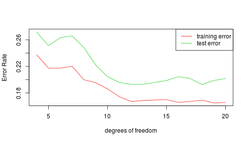
Let’s glance at the composition of the best-performing spline basis functions.
best <- which.min(errors[, 2])
df <- df[best]

# Visualize the best spline basis
h <- ns(f, df = df)
plot(f, h[, 1], type = "l", main = "Spline Basis Functions", xlab = "frequency",
    ylab = "h")
for (i in 2:df) {
    lines(f, h[, i], col = i)
}
Comparison
The regularized logistic fit outperformed the raw fit in predicting test data. The only exception was when using 4 degrees of freedom, which presumably did too much regularizing. The raw fit, however, performed better on the training data because it has so many parameters that it overfits.
M <- rbind(raw.errors, errors)
colnames(M) <- c("training error", "test error")
rownames(M)[1] <- "raw"
M


##     training error test error
## raw         0.1047     0.2485
## 4           0.2378     0.2719
## 5           0.2175     0.2515
## 6           0.2175     0.2632
## 7           0.2204     0.2661
## 8           0.2000     0.2485
## 9           0.1956     0.2222
## 10          0.1862     0.2047
## 11          0.1745     0.1959
## 12          0.1673     0.1930
## 13          0.1687     0.1930
## 14          0.1695     0.1959
## 15          0.1702     0.1988
## 16          0.1658     0.2047
## 17          0.1673     0.2018
## 18          0.1695     0.1930
## 19          0.1651     0.1988
## 20          0.1658     0.2018
All Five Phonemes
Next, I repeat the process, this time considering all five phonemes.
Raw Data
The following code relies on lr.predict which can be found elsewhere.
library(nnet)

lma <- multinom(g ~ ., x.train, MaxNWts = 1500)

# Find training and test error rates
yhat.train <- lr.predict(lma, x.train)
yhat.test <- lr.predict(lma, x.test)
raw.errors <- c(mean(yhat.train != x.train$g), mean(yhat.test != x.test$g))
Using Splines
For simplicity, I will only use the spline basis that worked best from before.
h <- H[[best]]
derived.train <- data.frame(as.matrix(x.train[, -r]) %*% h)
derived.train$g <- x.train$g

# Perform logistic regression on regularized data
lma <- multinom(g ~ ., derived.train)

# Find training and test error rates
yhat.train <- lr.predict(lma, derived.train)

derived.test <- data.frame(as.matrix(x.test[, -r]) %*% h)
derived.test$g <- x.test$g
yhat.test <- lr.predict(lma, derived.test)

errors <- c(mean(yhat.train != x.train$g), mean(yhat.test != x.test$g))
Comparison
The regularized logistic fit again outperformed the raw fit in predicting test data. And again, the raw fit worked better on the training data because of overfitting.
M <- rbind(raw.errors, errors)
colnames(M) <- c("training error", "test error")
rownames(M) <- c("raw", paste("reg df =", df))
M


##             training error test error
## raw                0.04103    0.09756
## reg df = 12 0.06654 0.07871blog comments powered by Disqus