$\newcommand{\E}{\mathbb{E}}$
$\newcommand{\I}{\mathbb{I}}$
$\renewcommand{\P}{\mathbb{P}}$
$\newcommand{\V}{\mathbb{\text{Var}}}$

Assume $X$ and $Y$ are each standard normal, and they have correlation coefficient $\rho$. Find the expectation of $X^2Y^2$.

First, consider the properties of $Y$ for a fixed $X$. In such a case, we have a simple linear model, and we know that $\E [Y \vert X] = \rho X$. Furthermore, $\rho^2$ represents the proportion of variation in $Y$ that is explained by $X$, so the proportion unexplained is

\begin{align*} \frac{\V [Y | X]}{\V Y} &= 1-\rho^2\\ \Rightarrow& \V [Y | X] = 1-\rho^2 \end{align*}

Also, note that $\E X^4 = 3$. This can be established by taking the fourth derivative of the standard normal moment generating function $e^{t^2/2}$ and evaluating it at $t=0$.

Now, we can use iterated expectation to derive the result.

\begin{align*} \E X^2 Y^2 &= \E \E [X^2 Y^2 | X]\\ &= \E X^2 \E [Y^2 | X]\\ &= \E X^2 \left( \E [Y | X]^2 + \V [Y | X] \right)\\ &= \E X^2 \left( (\rho X)^2 + (1-\rho^2) \right)\\ &= \rho^2 \E X^4 + (1-\rho^2) \E X^2\\ &= \rho^2 (3) + (1-\rho^2) (1)\\ &= 2\rho^2 + 1 \end{align*}

A simulation confirms our conclusion.

library(MASS)
n <- 10000
mu <- c(0, 0)

rho <- seq(-1, 1, by = 0.1)
results <- rep(NA, length(rho))
for (i in 1:length(rho)) {
    Sigma <- matrix(c(1, rho[i], rho[i], 1), nrow = 2)
    m <- mvrnorm(n, mu, Sigma)
    results[i] <- mean(m[, 1]^2 * m[, 2]^2)
}
plot(rho, results, ylab = expression(paste("Mean of  ", X^2, Y^2)),
     main = "Simulation Results and Theoretical Curve", xlab = expression(rho))
lines(rho, 2 * rho^2 + 1, col = 2)
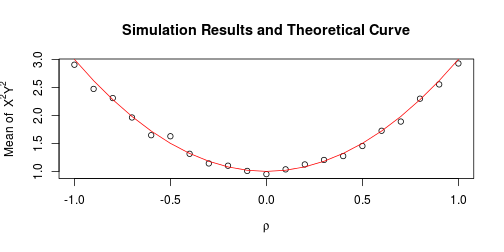
plot of chunk unnamed-chunk-1

Generalization

We can easily extend this result to the more general case of nonstandard normality. Assume $A \sim N(\mu_A, \sigma_A^2)$ and $B \sim N(\mu_B, \sigma_B^2)$ and they have correlation coefficient $\rho$. Then we can equivalently reexpress them as $A = \mu_A + \sigma_A X$ and $B = \mu_B + \sigma_B Y$ for some standard normal $X$ and $Y$ with correlation $\rho$.

We will also need to find a couple more expectations along the way.

\begin{align*} \E XY &= \E \E [XY | X]\\ &= \E X \E [Y | X]\\ &= \E X (\rho X)\\ &= \rho \E X^2\\ &= \rho \end{align*}

And

\begin{align*} \E X^2Y &= \E \E [X^2Y | X]\\ &= \E X^2 \E [Y | X]\\ &= \E X^2 (\rho X)\\ &= \rho \E X^3\\ &= 0 \end{align*}

Likewise, by symmetry, $\E XY^2 = 0$. Finally, we have all the pieces we need to attack the problem.

\begin{align*} \E A^2 B^2 &= \E \left( \mu_A + \sigma_A X \right)^2 \left( \mu_B + \sigma_B Y \right)^2\\ &= \E \left( \mu_A^2 + 2 \mu_A \sigma_A X + \sigma_A^2 X^2 \right) \left( \mu_B^2 + 2 \mu_B \sigma_B Y + \sigma_B^2 Y^2 \right)\\ &= \E \left[ \mu_A^2 \mu_B^2 + 2 \mu_A^2 \mu_B \sigma_B Y + \mu_A^2 \sigma_B^2 Y^2 + 2 \mu_A \mu_B^2 \sigma_A X + 4 \mu_A \mu_B \sigma_A \sigma_B XY + 2 \mu_A \sigma_A \sigma_B^2 XY^2 + \mu_B^2 \sigma_A^2 X^2 + 2 \mu_B^2 \sigma_A^2 \sigma_B X^2Y + \sigma_A^2 \sigma_B^2 X^2 Y^2 \right]\\ &= \mu_A^2 \mu_B^2 + 2 \mu_A^2 \mu_B \sigma_B (0) + \mu_A^2 \sigma_B^2 (1) + 2 \mu_A \mu_B^2 \sigma_A (0) + 4 \mu_A \mu_B \sigma_A \sigma_B (\rho) + 2 \mu_A \sigma_A \sigma_B^2 (0) + \mu_B^2 \sigma_A^2 (1) + 2 \mu_B^2 \sigma_A^2 \sigma_B (0) + \sigma_A^2 \sigma_B^2 (2\rho^2 + 1)\\ &= \mu_A^2 \mu_B^2 + \mu_A^2 \sigma_B^2 + 4 \mu_A \mu_B \sigma_A \sigma_B \rho + \mu_B^2 \sigma_A^2 + \sigma_A^2 \sigma_B^2 (2\rho^2 + 1)\\ \end{align*}


blog comments powered by Disqus

Published

15 March 2013

Tags