Comparing Classification Algorithms for Handwritten Digits Math, CS, Data
This is a simple exercise comparing several classification methods for identifying handwritten digits. The data are summarized on a prior post. Last time, I only considered classifying the digits “2” and “3”. This time I keep them all.
# Read in the training data
X.train <- read.table(gzfile("zip.train.gz"))
names(X.train)[1] <- "digit"
X.train$digit <- as.factor(X.train$digit)

# Read in the test data
X.test <- read.table(gzfile("zip.test.gz"))
names(X.test)[1] <- "digit"
X.test$digit <- as.factor(X.test$digit)
To compare methods, I rely a couple of utility functions which.response and crossval, which can be found elsewhere.
k-Nearest Neighbors
In order to cross-validate the results for a range of $k$ values, I will use a helper function.
knn.range <- function(formula, train, new, k.range) {
    # Performs a k-nearest neighbors classification for a range of k values.
    r <- which.response(formula, train)
    cl <- train[, r]
    all <- sort(unique(cl))
    train <- as.matrix(train[, -r])
    # If the response variable is in the new (test) data, remove it
    try({
        r.new <- which.response(formula, new)
        new <- new[, -r.new]
    }, silent = T)
    new <- as.matrix(new)
    results <- foreach(k = k.range, .combine = cbind) %do% {
        g <- knn(train, new, cl, k)
        return(g)
    }
    return(results)
}
Using the crossval function, along with knn.range, I try $k \in $ {$1, 2, 5, 10$} to look for a general trend.
library(foreach)
library(class)

k <- c(1, 2, 5, 10)
k.errors <- crossval(digit ~ ., X.train, K = 5, method = knn.range, k.range = k)

plot(k, k.errors, col = 2, ylab = "Error Rate",
     main = "k-NN Cross-validation Results")
lines(k, k.errors, col = 2, lty = 2)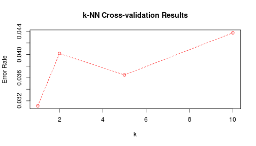
k <- k[which.min(k.errors)]I will now try the best $k$ on my training and my test data and record the error rates. The training error rate should be trivially zero when using $k=1$ nearest neighbors, as long as there are no exact ties belonging different classes. In this case, the probability of that is negligible.
yhat.train <- knn.range(digit ~ ., X.train, X.train, k)
yhat.test <- knn.range(digit ~ ., X.train, X.test, k)
knn.error <- c(mean(yhat.train != X.train$digit), mean(yhat.test != X.test$digit))

# What does k-NN mix up the most?
table(X.test$digit, yhat.test)


##    yhat.test
##       0   1   2   3   4   5   6   7   8   9
##   0 355   0   2   0   0   0   0   1   0   1
##   1   0 255   0   0   6   0   2   1   0   0
##   2   6   1 183   2   1   0   0   2   3   0
##   3   3   0   2 154   0   5   0   0   0   2
##   4   0   3   1   0 182   1   2   2   1   8
##   5   2   1   2   4   0 145   2   0   3   1
##   6   0   0   1   0   2   3 164   0   0   0
##   7   0   1   1   1   4   0   0 139   0   1
##   8   5   0   1   6   1   1   0   1 148   3
##   9   0   0   1   0   2   0   0   4   1 169
Linear Discriminant Analysis
LDA assumes that the various classes have the same covariance structure. The data cloud within each group should have the same basic shape. We cannot see the 256-dimensional data cloud, but we can visualize any two-dimensional projection of it, which should have that same property. The first two principal components for a sample of the data are plotted below.
s <- sample(1:nrow(X.train), 500)
p <- princomp(X.train[s, -1])
# Approximate proportion of variance in first two PCs
as.numeric((p$sd[1]^2 + p$sd[2]^2)/sum(p$sd^2))


## [1] 0.2642


plot(p$scores[, 1], p$scores[, 2], col = X.train$digit[s], xlab = "First PC",
     ylab = "Second PC", main = "Principal Component Scores")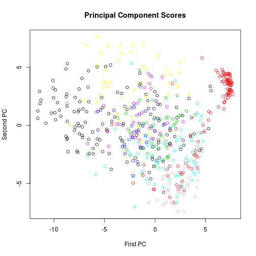
The assumption of equal covariance structures is not plausible. We will try LDA anyway for comparison to the other methods.
library(MASS)

z <- lda(digit ~ ., X.train)

# Find training and test error rates
yhat.train <- predict(z, X.train)$class
yhat.test <- predict(z, X.test)$class
lda.error <- c(mean(yhat.train != X.train$digit), mean(yhat.test != X.test$digit))

# What does LDA mix up the most?
table(X.test$digit, yhat.test)


##    yhat.test
##       0   1   2   3   4   5   6   7   8   9
##   0 342   0   0   4   3   1   5   0   3   1
##   1   0 251   0   2   5   0   3   0   1   2
##   2   7   2 157   4  12   2   1   1  12   0
##   3   3   0   3 142   3   9   0   1   4   1
##   4   1   4   6   0 174   0   2   2   1  10
##   5   6   0   0  16   3 125   0   0   5   5
##   6   1   0   3   0   3   3 157   0   3   0
##   7   0   1   0   2   7   0   0 129   1   7
##   8   5   0   2  11   7   4   0   0 135   2
##   9   0   0   0   0   4   0   0   5   3 165
Quadratic Discriminant Analysis
QDA discards the equal covariance assumption of LDA, but it estimates so many parameters that it has a high variance. Another drawback is that QDA algorithms are susceptible errors, as seen below.
z <- qda(digit ~ ., X.train)


## Error: rank deficiency in group 0


# Need to jitter the data to avoid exact multicolinearity

X.train.J <- X.train
X.train.J[, -1] <- apply(X.train[, -1], 2, jitter)
z <- qda(digit ~ ., X.train.J)

# Find training and test error rates
yhat.train <- predict(z, X.train)$class
yhat.test <- predict(z, X.test)$class
qda.error <- c(mean(yhat.train != X.train$digit), mean(yhat.test != X.test$digit))

# What does QDA mix up the most?
table(X.test$digit, yhat.test)


##   yhat.test
##      0   1   2   3   4   5   6   7   8   9
##  0 333   0  18   3   1   0   0   0   4   0
##  1   0 248   3   0   2   0   5   0   6   0
##  2   3   0 181   6   1   1   0   0   6   0
##  3   3   0   4 141   0   6   0   0  12   0
##  4   1   1  10   2 155   1   0   1   2  27
##  5   4   0   1   6   1 135   1   0  10   2
##  6   2   0  12   0   2   8 143   0   3   0
##  7   0   1   1   6   6   0   0 126   2   5
##  8   4   0  14  16   0   7   0   0 121   4
##  9   0   1   1   3   8   0   0   2   6 156
Regularized Discriminant Analysis
Technically, it’s redundant to do RDA in addition to LDA and QDA, because LDA and QDA are special cases of it. I could have just started with RDA, letting the $\lambda$ parameter vary over $[0, 1]$. In the klaR package’s rda function, $\lambda$ represents the amount of weight given to the pooled covariance matrix. Because I have already looked at $\lambda=1$ (LDA) and $\lambda=0$ (QDA), I will use cross-validation for range of $\lambda$ values between these extremes. My helper function rda.predict comes in handy.
Just like QDA, RDA will have problems with exactly multicolinear columns, so we will reuse the jittered data.
rda.predict <- function(formula, data, new, lambda, ...) {
    results <- foreach(l = lambda, .combine = cbind) %do% {
        z <- rda(formula, data, lambda = l, ...)
        return(predict(z, new)$class)
    }
    return(results)
}

library(klaR)

lambda <- seq(0.05, 0.95, 0.1)
r.errors <- crossval(digit ~ ., X.train.J, K = 5, method = rda.predict,
                     lambda = lambda, gamma = 0, crossval = F)
lambda <- lambda[which.min(r.errors)]
Now, I can use the best-performing $\lambda$ to try classifying the full training and test data.
z <- rda(digit ~ ., X.train.J, gamma = 0, lambda = lambda, crossval = F)

# Find training and test error rates
yhat.train <- predict(z, X.train)$class
yhat.test <- predict(z, X.test)$class
rda.error <- c(mean(yhat.train != X.train$digit), mean(yhat.test != X.test$digit))

# What does RDA mix up the most?
table(X.test$digit, yhat.test)


##    yhat.test
##       0   1   2   3   4   5   6   7   8   9
##   0 343   0   1   4   3   1   4   0   2   1
##   1   0 252   2   0   5   0   2   0   1   2
##   2   6   1 169   6   4   1   1   1   9   0
##   3   2   0   5 142   1   7   0   3   5   1
##   4   0   3   6   0 175   0   3   2   1  10
##   5   5   0   0   9   1 137   0   0   4   4
##   6   1   0   4   0   3   2 157   0   3   0
##   7   0   0   1   1   6   0   0 133   0   6
##   8   4   0   2   7   4   3   0   0 145   1
##   9   0   0   0   0   3   0   0   4   3 167
Logistic Regression
Finally, logistic regression makes fewer assumptions on the data. Let’s see how it does by using the nnet package’s multinom function and my lr.predict helper function.
lr.predict <- function(lr, data) {
    # Predicts the classes of the rows of data, based on a logistic regression
    # multinom object (from package 'nnet').  If response variable is in data,
    # remove it.
    formula <- lr$call$formula
    try({
        r <- which.response(formula, data)
        data <- data[, -r]
    }, silent = T)
    # Find probability values for each data row
    a <- 1L + (1L:length(lr$vcoefnames))
    coef <- matrix(lr$wts, nrow = lr$n[3L], byrow = TRUE)[-1L, a, drop = FALSE]
    # (above line of code is from nnet:::summary.multinom)
    X <- cbind(1, as.matrix(data))
    p <- exp(X %*% t(coef))
    baseline <- apply(p, 1, function(v) return(1/(1 + sum(v))))
    p <- baseline * p
    p <- cbind(baseline, p)
    # Find class with highest probability
    indices <- apply(p, 1, which.max)
    classes <- sapply(indices, function(i) return(lr$lev[i]))
    return(classes)
}

library(nnet)

z <- multinom(digit ~ ., X.train, MaxNWts = 3000)

# Find training and test error rates
yhat.train <- lr.predict(z, X.train)
yhat.test <- lr.predict(z, X.test)
lr.error <- c(mean(yhat.train != X.train$digit), mean(yhat.test != X.test$digit))

# What does logistic regression mix up the most?
table(X.test$digit, yhat.test)


##    yhat.test
##       0   1   2   3   4   5   6   7   8   9
##   0 343   0   3   2   3   2   2   3   1   0
##   1   0 254   2   1   1   0   1   1   1   3
##   2   5   1 163   6   8   1   1   5   7   1
##   3   2   0   4 145   1   8   1   2   3   0
##   4   5   2   5   1 168   2   4   1   4   8
##   5   4   1   0   7   3 137   3   0   2   3
##   6   1   0   4   0   4   4 156   0   1   0
##   7   0   0   2   3   5   0   0 132   0   5
##   8   7   0   7   3   1   9   0   4 130   5
##   9   0   0   0   1   3   1   0   2   5 165
Comparing the Methods
error <- rbind(knn.error, lda.error, qda.error, rda.error, lr.error)
colnames(error) <- c("Training Error Rate", "Test Error Rate")
rownames(error) <- c(paste("KNN with k =", k), "LDA", "QDA",
                     paste("RDA with lambda =", lambda), "Logistic Regression")
error


##                        Training Error Rate Test Error Rate
## KNN with k = 1                   0.0000000         0.05630
## LDA                              0.0619942         0.11460
## QDA                              0.0220820         0.13353
## RDA with lambda = 0.95           0.0405980         0.09317
## Logistic Regression              0.0001372         0.10663
For this problem, k-nearest neighbors was the most successful in predicting the groups of the test data. This may have to do with the fact that it makes the fewest assumptions. The other (parametric) methods are based on models that may be inappropriate for this problem.
blog comments powered by Disqus