Spline Derivatives Math, CS, Data
I recently assisted a physicist with a simple data analysis issue. She had taken a series of measurements with an instrument at varying levels of some setting $\Omega$. The consecutive data points should be noisy about an underlying smooth curve. The physicist wanted to estimate the derivative of this curve at her data points.
Even without assuming any simple parametric structure to the curve, we can achieve this quite easily by using R’s built-in smooth.spline function.
The data has three columns: the predictor variable $\Omega$, and two columns (corresponding to real and imaginary parts) of response variables. The different values of $\Omega$ are spaced out evenly on a logarithmic scale. By log-transforming these $\Omega$ values, we can get evenly spaced data points; this will make the spline fit work better.
filename <- "NaCl_Omega.ReZ.ImZ.csv"
X <- read.csv(filename, header = F)
O <- X[, 1]
R <- X[, 2]
I <- X[, 3]

# Transform Omega values
o <- log(O)

### Reals ###

# Fit smooth curve for Reals
par(mfrow = c(1, 2))
plot(o, R, xlab = expression(log[n] ~ Omega), ylab = "Real",
     main = "Real Data with Spline Fit")
s <- smooth.spline(o, R)
lines(predict(s, o), col = 2, lwd = 2)

plot(O, R, xlab = expression(Omega), ylab = "Real",
     main = "Data with Spline Fit")
lines(O, s$y, col = 2, lwd = 2)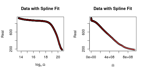
Now, the predict.smooth.spline method can give us the derivative of the fit curve at our chosen values. However, because of our natural logarithm transformation, these will be the derivatives with respect to $\log \Omega$. To get the derivatives with respect to $\Omega$, we simply need to divide these derivatives by $\Omega$ because
# Numerical derivatives
dy <- predict(s, o, deriv = 1)$y/O
outR <- log10(-dy)
plot(log10(O/2/pi), outR, xlab = expression(log[10] ~ Frequency),
     ylab = expression(log[10] ~ "(-d Real)"),
     main = "Derivative of Real Spline Fit")
Repeat for imaginary values.
### Imaginaries ###

# Fit smooth curve for Imaginaries
par(mfrow = c(1, 2))
plot(o, I, xlab = expression(log[n] ~ Omega), ylab = "Imaginary",
     main = "Imaginary Data with Spline Fit")
s <- smooth.spline(o, I)
lines(o, s$y, col = 2, lwd = 2)

plot(O, I, xlab = expression(Omega), ylab = "Imaginary",
     main = "Data with Spline Fit")
lines(O, s$y, col = 2, lwd = 2)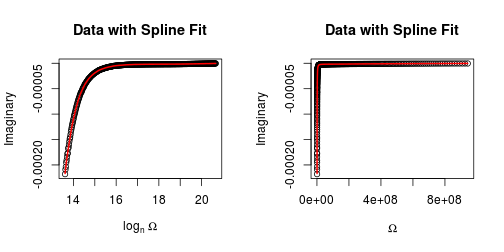
# Numerical derivatives
dy <- predict(s, o, deriv = 1)$y/O
outI <- log10(dy)
plot(log10(O/2/pi), outI, xlab = expression(log[10] ~ Frequency),
     ylab = expression(log[10] ~ "(d Imaginary)"),
     main = "Derivative of Imaginary Spline Fit")
Automating it with Rscript
The physicist will be gathering much more data of this type. The following R script (named ORIspline.R) will allow her to compute the derivative estimates easily on that future data.
Example command line usage: Rscript ORIspline.R NaCl_Omega.ReZ.ImZ.csv
Notice that the name of the file to be analyzed is passed in as a command-line parameter.
filename <- commandArgs(T)[1]

X <- read.csv(filename, header = F)
O <- X[, 1]
R <- X[, 2]
I <- X[, 3]

# Transform Omega values
o <- log(O)

### Reals ###
s <- smooth.spline(o, R)
dy <- predict(s, o, deriv = 1)$y/O
outR <- log10(-dy)

### Imaginaries ###
s <- smooth.spline(o, I)
dy <- predict(s, o, deriv = 1)$y/O
outI <- log10(dy)

# Create csv file
final <- cbind(O, outR, outI)
colnames(final) <- c("Omega", "log10 -dRe", "log10 dIm")
write.csv(final, paste0("derivatives_", filename), row.names = F)blog comments powered by Disqus