The Black-Scholes Model

$\newcommand{\E}{\mathbb{E}} \renewcommand{\P}{\mathbb{P}}$

In 1973, Fisher Black and Myron Scholes solved a fundamental problem of mathematical finance in their paper The Pricing of Options and Corporate Liabilities. They discovered a model for stocks that determined a single price for options. Furthermore, they derived a formula for computing that price. Their mathematical breakthrough quickly spread beyond academia and revolutionized the world of finance and investment. This article describes the assumptions of the Black-Scholes model and derives the Black-Scholes formula for determining option prices, following the steps from An Elementary Introduction to Mathematical Finance by Sheldon Ross.

Model Assumptions

Geometric Brownian Motion

The Black-Scholes model assumes that stock prices are Geometric Brownian Motions (GBM). A GBM is a stochastic process whose natural logarithm is a Brownian Motion.

Definition

If we have a Brownian Motion

\begin{align*} \log U(t) = b_0 + \mu t + \sigma W_t \end{align*}

where $W_t$ is $N(0,t)$, then $U$ is a GBM. Consider the distribution of $U(t)$. Let $u_0 = e^{b_0}$. Then $U(t) = u_0 e^{\mu t + \sigma W_t}$. We can compute the expected value using the fact that $W_t$ has a distribution $N(0,t)$.

\begin{align*} \E U(t) &= \E [u_0 e^{\mu t + \sigma W_t}]\\ &= \int u_0 e^{\mu t + \sigma x} \frac{1}{\sqrt{2\pi t}}\, e^{-x^2/2t} dx\\ &= u_0 e^{\mu t} \int \frac{1}{\sqrt{2\pi t}}\, e^\frac{-x^2+2t\sigma x}{2t} dx\\ &= u_0 e^{\mu t} \int \frac{1}{\sqrt{2\pi t}}\, e^\frac{-x^2+2t\sigma x - t^2\sigma^2 + t^2\sigma^2}{2t} dx\\ &= u_0 e^{\mu t} e^{t^2\sigma^2/2t} \int \frac{1}{\sqrt{2\pi t}}\, e^\frac{-x^2+2t\sigma x - t^2\sigma^2}{2t} dx\\ &= u_0 e^{\mu t} e^{t \sigma/2} (1)\\ &= u_0 e^{t(\mu + \sigma/2)} \end{align*}

so $U$ has an initial value of $u_0$ and its mean grows exponentially over time with a rate of $\mu + \sigma/2$.

Justification

Stock prices do indeed have the “look” of Brownian Motion. But regular Brownian Motion can take negative values, whereas GBM cannot. Because stock prices are bounded below by zero, GBM seems more appropriate in this case. In addition, market analysts believe that the percentage change of a stock on any given day is normally distributed rather than the actual amount of change. For instance, assuming GBM, a stock price moving from \$9 to \$10 is as likely as that stock price moving from \$90 to \$100. Assuming ordinary Brownian Motion, a stock price moving from \$9 to \$10 is as likely as that stock price moving from \$90 to \$91. Based on our intuitions as well as empirical observations, the GBM model is more appropriate in this regard as well.

Construction

There is a common algorithm for constructing Standard Brownian Motion on $(0, T)$. You take $U(0) = 0$ to be your first point, and generate $U(T)$ from $N(0, T)$. Next, generate a BM value at the midpoint of your interval conditional on the values at the endpoints. Repeat this process recursively on each new subinterval. By following the algorithm for a finite number of steps, you can simulate approximate Brownian Motion.

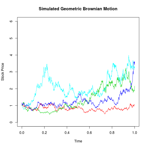
By simulating Brownian Motion and exponentiating the result, we can simulate GBM. My code below generates four simulated examples of GBM. In each case, $2^{10}$ points were generated for a Brownian Motion starting at (0,0) with drift factor 1 and noise factor 1. Exponentiation of the results gives us GBMs.

BMrecur <- function(x, y, sigma) {
    m <- length(x)
    mid <- (m + 1)/2
    delta <- x[m] - x[1]
    y[mid] <- (y[1] + y[m])/2 + rnorm(1, sd = sigma * sqrt(delta)/2)
    if (m <= 3) {
        return(y[mid])
    } else {
        return(c(BMrecur(x[1:mid], y[1:mid], sigma), y[mid],
                 BMrecur(x[mid:m], y[mid:m], sigma)))
    }
}

GenerateBM <- function(end = 1, initial = 0, mu = 0, sigma = 1, log2n = 10,
                       geometric = F) {
    n <- 2^log2n
    x <- end * (0:n)/n
    final <- initial + mu * end + rnorm(1, sd = sigma * sqrt(end))
    y <- c(initial, rep(NA, n - 1), final)
    y[2:n] <- c(BMrecur(x, y, sigma))
    if (geometric) y <- exp(y)
    return(cbind(x, y))
}


plot(c(0, 1), c(0, 6), type = "n", main = "Simulated Geometric Brownian Motion", 
    xlab = "Time", ylab = "Stock Price")
set.seed(3)
for (i in 1:4) {
    lines(GenerateBM(mu = 1, geometric = T), col = i + 1)
}

plot of chunk unnamed-chunk-2

There is another, more direct, way to construct a GBM, as described in section 3.2 of Ross. Let $\Delta$ denote a small time-step and assume that that at each time-step a stock price $U(t)$ either rises by a factor of $u := e^{\sigma\,\sqrt{\Delta}}$ or falls by a factor of $d := e^{-\sigma\,\sqrt{\Delta}}$. The probability of rising is

\begin{align*} p := \frac{1}{2}\left( 1 + \frac{\mu}{\sigma}\,\sqrt{\Delta} \right) \end{align*}

If the stock starts at a price $u_0$, then after $n$ time-steps the price of the stock will be

\begin{align*} U(n\Delta) = u_0 u^{X_n} d^{n-X_n} = u_0 d^n \left( \frac{u}{d} \right)^{X_n} \end{align*}

where $X_n$ is the number of times the stock rose, which has a Binomial$(n,p)$ distribution. Taking the natural logarithm,

\begin{align*} \log U(n\Delta) &= \log u_0 + n \log d + X_n \log (u/d)\\ &= \log u_0 + n \log e^{-\sigma\,\sqrt{\Delta}} + X_n \log (e^{\sigma\,\sqrt{\Delta}} / e^{-\sigma\,\sqrt{\Delta}})\\ &= \log u_0 - n \sigma \, \sqrt{\Delta} + X_n (2 \sigma \, \sqrt{\Delta}) \end{align*}

Now we make some manipulations to standardize $X_n$.

\begin{align*} \log U(n\Delta) &= \log u_0 - n \sigma \, \sqrt{\Delta} + (X_n - np + np) (2 \sigma \, \sqrt{\Delta})\\ &= \log u_0 - n \sigma \, \sqrt{\Delta} + (X_n - np) (2 \sigma \, \sqrt{\Delta}) + 2 np \sigma \sqrt{\Delta}\\ &= \log u_0 - n \sigma \, \sqrt{\Delta} + (X_n - np) (2 \sigma \, \sqrt{\Delta}) + 2 n \left( \frac{1}{2}\left( 1 + \frac{\mu}{\sigma}\sqrt{\Delta} \right) \right) \sigma \sqrt{\Delta}\\ &= \log u_0 + \mu n \Delta + (X_n - np) (2 \sigma \, \sqrt{\Delta})\\ &= \log u_0 + \mu n \Delta + (\sqrt{np(1-p)})\left(\frac{X_n - np}{\sqrt{np(1-p)}}\right) (2 \sigma \, \sqrt{\Delta})\\ &= \log u_0 + \mu n \Delta + \left(\frac{\sqrt{n}\,\sqrt{\sigma^2 + \mu^2 \Delta}}{2\sigma}\right)\left(\frac{X_n - np}{\sqrt{np(1-p)}}\right) (2 \sigma \, \sqrt{\Delta})\\ &= \log u_0 + \mu n\Delta + (\sqrt{\sigma^2 + \mu^2 \Delta}) \sqrt{n\Delta} \left(\frac{X_n - np}{\sqrt{np(1-p)}}\right) \end{align*}

If we now let $\Delta \rightarrow 0$ and $n \rightarrow \infty$ such that $t := n\Delta$ is fixed, we get

\begin{align*} \log U(t) &= \log u_0 + \mu t + \sigma \sqrt{t} Z \end{align*}

where $Z := \lim (X_n-np)/\sqrt{np(1-p)}$ has a standard normal distribution, by the central limit theorem. It is clear that this process has “the right kind of independence,” so $\log U$ is a Brownian Motion with initial position $\log u_0$, drift $\mu$, and volatility $\sigma$. Therefore, $U$ is a GBM. This construction will be used to derive the Black-Scholes formula below.

Arbitrage

Second, we assume that there should be no opportunity for arbitrage. “Arbitrage” is an investment strategy that guarantees the investor a rate of return greater than the risk-free interest rate.

According to the Arbitrage Theorem (see Ross section 6.3 for a proof), if there is no opportunity for arbitrage, then there is a probability vector $\mathbb{P} := (p_1,\ldots,p_m)$ corresponding to the $m$ possible outcomes such that an investor’s expected return (above the risk-free rate) is zero regardless of his strategy. This theorem provides a method that is sometimes useful in option price calculations. First, pick one possible investment strategy. Next, find a probability vector such that the expected return is zero. If that probability vector is unique, then it must make all possible strategies zero. Using this fact may allow you to solve for the option price.

One particular instance of this method (Ross section 6.2) is the case where a stock price comprises a sequence of $n$ Bernoulli steps (paralleling somewhat our construction of GBM). Let $U(k)$ be the stock price after $k$ steps, $u$ be the factor that it rises by, and $d$ be the factor that it falls by, and let $r$ be the risk-free rate. Let $X := (X_1,\ldots,X_n)$ be a random vector of indicator functions with $X_j = 1$ if the stock price rose by $u$ during step $j$ and $X_j = 0$ if the stock price fell by $d$ during step $j$. Consider the following strategy. First choose some $i \in {1,\ldots,n}$ and some particular vector $(x_1,\ldots,x_{i-1})$ of zeros and ones. Now, if and only if $(X_1,\ldots,X_n) = (x_1,\ldots,x_n)$ (call this event $A$), you buy one unit of stock at the beginning of period $i$ and sell it back at the end of that period. Otherwise, if the first $i-1$ observations do not match your pre-specified pattern, you do nothing. With this strategy, your overall expected gain is

\begin{align*} \E(\text{Gain}) &= \P(A) \E(\text{Gain}|A) + \P(A^c) \E(\text{Gain}|A^c)\\ &= \P(A) \E(\text{Gain}|A) + \P(A^c) (0)\\ &= \P(A) \E(\text{Gain}|A)\\ &= \P(A) [\P(X_i=1) \E(\text{Gain}|A,X_i=1) + \P(X_i=0) \E(\text{Gain}|A,X_i=0)]\\ &= \P(A) \left[\P(X_i=1) \left( \frac{u U(i-1)}{1+r} - U(i-1)\right) + \P(X_i=0) \left( \frac{d U(i-1)}{1+r} - U(i-1)\right)\right]\\ &= \P(A) \left[p\left( \frac{u U(i-1)}{1+r} \right) + (1-p)\left( \frac{d U(i-1)}{1+r} \right) - U(i-1)\right] \end{align*}

for some “success” probability $p$ corresponding to the $i$th step, given $A$. Setting this gain equal to zero and solving for $p$ gives

\begin{align*} p &= \frac{1+r-d}{u-d} \end{align*}

In fact, because $i$ is arbitrary, the only probability vector that can make all bets of this type fair must have this same success probability at each step. Because $(x_1,\ldots,x_{i-1})$ is arbitrary, the steps must be independent. So the only probability distribution for which all of these bets are fair must correspond to a sequence of $n$ independent Bernoulli steps. By the Arbitrage Theorem, we can make the broader statement that this probability distribution will actually be fair for all possible strategies.

Now, assume that for a price of $C$, we can purchase the option to buy the stock $n$ steps from now at a price of $K$. Assuming no arbitrage is possible, the distribution we found above must make the expected payout of the option exactly equal to its price. If $U(n)$ is greater than $K$, then the value of the option is the difference, otherwise the option’s value is zero.

\begin{align*} C &= \frac{\E[(U(n)-K)^+]}{(1+r)^n}\\ &= \frac{\E[(u^Yd^{n-Y}U(0)-K)^+]}{(1+r)^n} \end{align*}

where $Y := \sum X_i \sim$ Binomial$(n,p)$. This result will be employed below to derive the Black-Scholes formula.

Other Assumptions

A call option is the right to purchase a stock at some time in the future at pre-specified price called a “strike price.” We assume that options will not be exercised before they expire.

We also assume that there is a constant risk-free interest rate. This is the interest rate at which money could be borrowed or saved (in a savings account, for example) with certainty. We assume that any amount of stock can be bought or sold at no cost. Finally, we assume that the stock does not pay dividends.

The Formula

Definitions

Let

\begin{align*} U(t) &:= \text{stock price (GBM indexed by time $t$)}\\ K &:= \text{strike price}\\ T &:= \text{expiration time}\\ r &:= \text{nominal risk-free rate}\\ \mu &:= \text{drift rate of $U$}\\ \sigma &:= \text{volatility of $U$}\\ u_0 &:= \text{initial price of $U$} \end{align*}

Derivation

Ross (sections 7.2 and 7.5) outlines the following derivation of the Black-Scholes formula.

We start with $U_n$, an $n$-stage binomial model from the “Construction” section with $u$ and $d$ as defined before, but consider the first three terms of their Taylor expansions. (We will write $T/n$ for $\Delta$.)

\begin{align*} u &= e^{\sigma \sqrt{T/n}}\, = 1 + \sigma \sqrt{T/n} + \sigma^2 T/2n\\ d &= e^{-\sigma \sqrt{T/n}} = 1 - \sigma \sqrt{T/n} + \sigma^2 T/2n\\ \end{align*}

We know from the “Arbitrage” section that the only success probability that makes this process fair for all bets is

\begin{align*} p &= \frac{1+rT/n-d}{u-d}\\ &\approx \frac{1 + rT/n - (1 - \sigma \sqrt{T/n} + \sigma^2 T/2n)}{(1 + \sigma \sqrt{T/n} + \sigma^2 T/2n) - (1 - \sigma \sqrt{T/n} + \sigma^2 T/2n)}\\ &= \frac{\sigma \sqrt{T/n} - \sigma^2 T/2n + rt/n}{2\sigma \sqrt{T/n}}\\ &= \frac{1}{2}\left( 1 + \frac{r - \sigma^2 /2}{\sigma}\sqrt{T/n} \right) \end{align*}

Comparing this to the success probability in the “Construction” section, we can see that it has the exact same form. Therefore, in the limit, this process $U_n \rightarrow U$ is a GBM with drift parameter $\mu = r-\sigma^2$ and volatility parameter $\sigma$.

Furthermore, from the “Arbitrage” section, the price of an option should be

\begin{align*} C &= \lim \frac{\E[(U_n(T)-K)^+]}{(1+rT)^n}\\ &= e^{-rT} \E[(U(T)-K)^+]\\ &= e^{-rT} \E[(U(T)-K) I] \qquad \text{with indicator } I := \{U(T)>K\}\\ &= e^{-rT} \E[U(T) I] - K e^{-rT} \E[I] \end{align*}

This GBM $U$ has the property that $U(T) = u_0 e^{(r-\sigma^2)T + \sigma \sqrt{T}\, Z}$ where $Z$ is standard normal. Now, let us compute each of the two expectations in the above expression separately.

\begin{align*} \E[I] &= \P (U(T) > K)\\ &= \P (u_0 e^{(r-\sigma^2)T + \sigma \sqrt{T}\, Z} > K)\\ &= \P (Z > \frac{\log(K/u_0) - (r-\sigma^2/2)T}{\sigma \sqrt{T}})\\ &= \P (Z > \sigma \sqrt{T} - \omega) \qquad \text{where } \omega := \frac{rT + \sigma^2T/2 - \log (K/u_0)}{\sigma \sqrt{T}}\\ &= \P (Z < \omega - \sigma \sqrt{T}) \qquad \text{by symmetry of $Z$}\\ &= \Phi (\omega - \sigma \sqrt{T}) \qquad \qquad \text{where $\Phi$ is the standard normal cdf} \end{align*}

Define $c := \sigma \sqrt{T} - \omega$. Because $I \equiv {Z > \sigma \sqrt{T} - \omega}$, we can integrate $U(T)$ from $c$ to $\infty$ to get the other expectation

\begin{align*} \E [U(T) I] &= \int_c^\infty u_0 e^{(r-\sigma^2)T + \sigma \sqrt{T}\, x} \frac{1}{\sqrt{2\pi}} e^{-x^2/2} dx\\ &= u_0 e^{(r-\sigma^2)T} \int_c^\infty e^{\sigma \sqrt{T}\, x} \frac{1}{\sqrt{2\pi}} e^{-x^2/2} dx\\ &= u_0 e^{(r-\sigma^2)T} \int_c^\infty \frac{1}{\sqrt{2\pi}} e^{-(x^2-2\sigma \sqrt{T}\, x)/2} dx\\ &= u_0 e^{(r-\sigma^2)T} \int_c^\infty \frac{1}{\sqrt{2\pi}} e^{-(x-\sigma \sqrt{T})^2/2} e^{\sigma^2T/2} dx \qquad \text{after completing the square}\\ &= u_0 e^{rT} \int_c^\infty \frac{1}{\sqrt{2\pi}} e^{-(x-\sigma \sqrt{T})^2/2} dx\\ &= u_0 e^{rT} \int_\omega^\infty \frac{1}{\sqrt{2\pi}} e^{-x^2/2} dx \qquad \qquad \qquad \text{shift leftward by } \sigma \sqrt{T}\\ &= u_0 e^{rT} \P (Z > \omega)\\ &= u_0 e^{rT} \Phi (\omega) \end{align*}

Finally, putting everything back together, the Black-Scholes formula is

\begin{align*} C(u_0,T,K,\sigma,r) &= u_0 \Phi(\omega) - K e^{-rT} \Phi(\omega - \sigma \sqrt{T})\\ \text{where } \omega &:= \frac{rT + \sigma^2T/2 - \log (K/u_0)}{\sigma \sqrt{T}} \end{align*}

Usage

One of the features of Black-Scholes that has made it so useful is that the variables determining the option price can be known quite accurately. In fact, four of the variables, (initial stock price, time to expiration, strike price, and risk-free rate) are “exactly” known. The only variable that must be estimated is the volatility of the stock, and this can be estimated with relatively high precision.

Esteemed by financial mathematicians and on-the-floor traders alike, the Black-Scholes formula is surely one of the most influential equations of all time. Lately, however, its use has been called into question somewhat, particularly in the wake of the financial crisis. Among other problems, the assumption that stock prices follow GBM leads us to predict far fewer outliers than we actually see in practice. A model with fatter tails would perhaps match the data better and help financial markets be more robust to crashes.

blog comments powered by Disqus

Published

28 December 2012

The Black-Scholes Model Math, CS, Data