Method of Types Math, CS, Data
This article summarizes the method of types, as presented in Chapter 11 of the Cover and Thomas (C&T) text Elements of Information Theory.
Types (Based on C&T Section 11.1)
Consider a sequence $X_1, \ldots, X_n$ of i.i.d. discrete random variables with alphabet $A = {a_1, \ldots, a_m}$. The distribution of $X_i$ comprises the probabilities $Q = (q_1, \ldots, q_m)$ corresponding to the alphabet. By definition, the probabilities satisfy $q_i \geq 0$ and $\sum q_i = 1$, meaning that $Q$ is limited to a bounded $(m-1)$-dimensional figure within $\R^m$, known as the probability simplex in $\R^m$.
This distribution is often estimated by the empirical distribution $\Px$. Component $i$ of $\Px$ is defined to be the proportion of times $a_i$ occurred in $\x$. Notice that this does not depend on the order of the occurrences but only on the number. In other words, any permutation of a given sequence maps to the same empirical distribution. This observation allows us to split the $m^n$ possible sequences into equivalence classes, known as “types.” The type class corresponding to a distribution $P$ is denoted $T(P)$.
Notice that $\Px$ has the same constraints as $Q$, so it must lie within the simplex as well. Furthermore, for any given $n$, there are only a finite number of possible values for $\Px$. Each component of $\Px$ must be representable by a fraction in $[0,1]$ with denominator $n$. Therefore, the possible values of $\Px$ form a grid within the simplex. For example, the possible empirical distributions in the $m=3$ case are displayed below. (I used Picasion to merge the pictures into a single animation.)
library(grid)

drawSimplex <- function() {
    # Draws the probability simplex for the alphabet of size 3
    grid.polygon(x = c(0, 1, 0.5), y = c(0, 0, 1))
    grid.text("p1=1", 0.5, 1.05)
    grid.text("p2=1", -0.03, -0.05)
    grid.text("p3=1", 1.03, -0.05)
}


for (n in 1:10) {
    png(paste(n, ".png", sep = ""), width = 400, height = 400)
    grid.newpage()
    pushViewport(viewport(x = 0.15, y = 0.15, w = unit(10, "cm"),
                          h = unit(10 * sqrt(3)/2, "cm"),
                          just = c("left", "bottom"),
                          xscale = c(0, n), yscale = c(0, n)))
    drawSimplex()
    grid.text("Possible Empirical Distributions", 0.5, 1.2,
              gp = gpar(fontsize = 20))
    grid.text(paste("n =", n), 0.04, 0.7, just = "left",
              gp = gpar(fontsize = 25, col = 2))
    for (i in 0:n) {
        x <- 0:(n - i) + i/2
        grid.circle(x, i, unit(0.015, "npc"), default.units = "native",
                    gp = gpar(col = 2, fill = 2))
    }
    popViewport(1)
    dev.off()
}
The number of possible empirical distributions can be computed exactly, but the following rough upper bound proves to be more convenient.
Theorem 1
The number of possible empirical distributions is bounded by $(n+1)^m$.
Proof
There are only $n+1$ fractions in $[0,1]$ with denominator $n$, and each of the $m$ components must take one of these values. There are only $(n+1)^m$ such possibilities. The subset of these that have components summing to 1 are the possible empirical distributions in the simplex. $\square$
The remaining theorems relate to entropy and relative entropies.
Theorem 2
The probability of any particular outcome $\x = (x_1, \ldots, x_n)$ is $2^{-n (H(\Px) + D(\Px \Vert Q))}$.
Proof
Let $N(a \vert \x)$ denote the number of occurrences of $a$ in $\x$. Then (from C&T page 350)
$\square$
Note that all outcomes in the same type class have the same probability. To illustrate entropy and relative entropies over the simplex, I wrote code to generate level curves for the $m=3$ case.
H <- function(p1, p2, p3 = 1 - p1 - p2, ...) {
    # Entropy of a discrete distribution
    p <- c(p1, p2, p3)
    return(-sum(log2(p^p)))
}

D <- function(p1, p2, p3 = 1 - p1 - p2, q1, q2, q3 = 1 - q1 - q2) {
    # Relative entropy between two discrete distributions
    p <- c(p1, p2, p3)
    q <- c(q1, q2, q3)
    return(sum(log2(p^p) - log2(q^p)))
}

HplusD <- function(...) {
    # Simplifies to -sum(p*log2(q))
    return(H(...) + D(...))
}

roots <- function(f, ..., a = 0, b = 1, r = (b - a)/100) {
    # Finds the roots of f on interior of (a, b) (they need to pass through 0)
    x <- seq(a + r, b - r, by = r)
    y <- sapply(x, f, ...)
    roots <- c()
    # Each time the sign changes, run uniroot on the interval
    for (i in 1:(length(x) - 1)) {
        if (sign(y[i + 1]) != sign(y[i])) {
            roots <- c(roots, uniroot(f, c(x[i], x[i + 1]), ...)$root)
        }
    }
    return(roots)
}

levelCurve <- function(f, ..., d) {
    # Assumes level curve is convex
    p2 <- seq(0.001, 0.999, by = 0.001)
    l <- length(p2)
    p1 <- rep(NaN, 2 * l)
    for (i in 1:l) {
        j <- 2 * l - i + 1
        z <- roots(function(x) f(x, p2 = p2[i], ...) - d, b = 1 - p2[i])
        if (length(z) == 2) {
            p1[i] <- min(z)
            p1[j] <- max(z)
        } else if (length(z) == 1) {
            z <- z[1]
            if (i == 1) {
                p1[i] <- z
                p1[j] <- z
            } else {
                # what is z closer to?
                if (is.na(p1[i - 1])) {
                  p1[j] <- z
                  p1[i] <- NA
                } else if (is.na(p1[j + 1])) {
                  p1[i] <- z
                  p1[j] <- NA
                } else if (abs(p1[i - 1] - z) > abs(p1[j + 1] - z)) {
                  p1[j] <- z
                  p1[i] <- NA
                } else {
                  p1[i] <- z
                  p1[j] <- NA
                }
            }
        }
    }
    p2 <- c(p2, rev(p2))
    keep <- !is.nan(p1)
    p1 <- p1[keep]
    p2 <- p2[keep]
    return(cbind(p1, p2))
}

simplexTransform <- function(p1, p2, p3 = 1 - p1 - p2) {
    # Returns the horizontal component of the point
    return(p1/2 + (1 - p2/(p2 + p3)) * (1 - p1))
}

drawCurves <- function(f, q1 = NA, q2 = NA, fstr, ds) {
    pushViewport(viewport(w = unit(10, "cm"), h = unit(10 * sqrt(3)/2, "cm")))
    drawSimplex()
    grid.text(paste("Level Curves of", fstr), 0.5, 1.13, gp = gpar(fontsize = 20))
    if (fstr != "H") {
        grid.text("Q", simplexTransform(q1, q2), q1, default.units = "native",
                  gp = gpar(col = 2))
    }
    for (d in ds) {
        l <- levelCurve(f, q1 = q1, q2 = q2, d = d)
        p1 <- l[, 1]
        p2 <- simplexTransform(l[, 1], l[, 2])
        m <- length(p1)
        grid.segments(p2, p1, p2[c(2:m, 1)], p1[c(2:m, 1)], gp = gpar(col = 3))
        position <- which.max(p1)
        grid.text(paste(fstr, "=", d, sep = ""), p2[position],
                  p1[position] - 0.04, gp = gpar(col = 4, fontsize = 10))
    }
    popViewport(1)
}
Based on Theorem 2, we can visualize the empirical distributions that correspond to equally probable outcomes. Below are plots of level curves for $H(\cdot)$, $D(\cdot \Vert Q)$, and $H(\cdot) + D(\cdot \Vert Q)$, using $Q = (3/6, 2/6, 1/6)$.
drawHD <- function(q1, q2) {
    pushViewport(viewport(x = 0, w = 0.5, h = 0.5, just = c("left", "bottom")))
    drawCurves(H, fstr = "H", ds = c(1.5, 1.25, 1))
    popViewport(1)
    pushViewport(viewport(x = 0.5, w = 0.5, h = 0.5, just = c("left", "bottom")))
    drawCurves(D, q1 = q1, q2 = q2, fstr = "D", ds = c(0.1, 0.3, 0.5))
    popViewport(1)
}

png("Q1.png", height = 700, width = 700)
grid.newpage()
drawHD(1/2, 1/3)
pushViewport(viewport(x = 0.25, y = 0, w = 0.5, h = 0.5,
             just = c("left", "bottom")))
drawCurves(HplusD, q1 = 1/2, q2 = 1/3, fstr = "H+D", ds = c(1.2, 1.6, 2))
popViewport(1)
dev.off()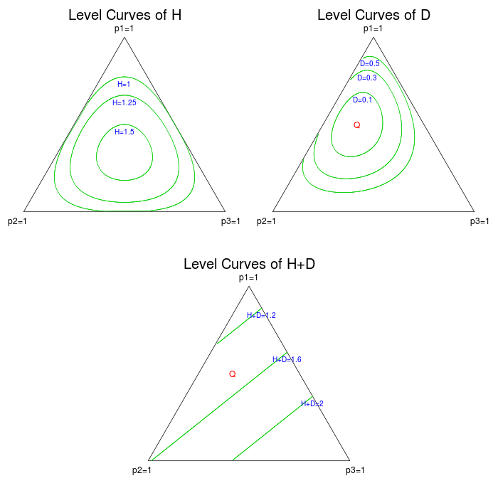
Note that lower values of $H+D$ correspond to exponentially higher probabilities. We should not be surprised to see that the level curves are line segments, because $H(P) + D(P \, \Vert Q)$ simplifies to
a linear combination of the components of $P$. Its level sets are represented by 2-dimensional planes in $\R^3$. A subset of these planes intersect the probability simplex, and those intersections form line segments.
Also, notice that in the $Q=(1/3,1/3,1/3)$ case, this expression is equal to $\log 3$ for all $P$. The level curves for this case are plotted below.
png("Q2.png", height = 700, width = 700)
grid.newpage()
drawHD(1/3, 1/3)
pushViewport(viewport(x = 0.25, y = 0, w = 0.5, h = 0.5,
             just = c("left", "bottom")))
pushViewport(viewport(w = unit(10, "cm"), h = unit(10 * sqrt(3)/2, "cm")))
drawSimplex()
grid.polygon(x = c(0, 1, 0.5), y = c(0, 0, 1), gp = gpar(fill = 3))
grid.text("Level Curves of H+D", 0.5, 1.13, gp = gpar(fontsize = 20))
grid.text("Q", simplexTransform(1/3, 1/3), 1/3, default.units = "native",
          gp = gpar(col = 2))
grid.text("H+D=1.585 everywhere", 0.5, 0.22, gp = gpar(col = 4, fontsize = 10))
popViewport(1)
popViewport(1)
dev.off()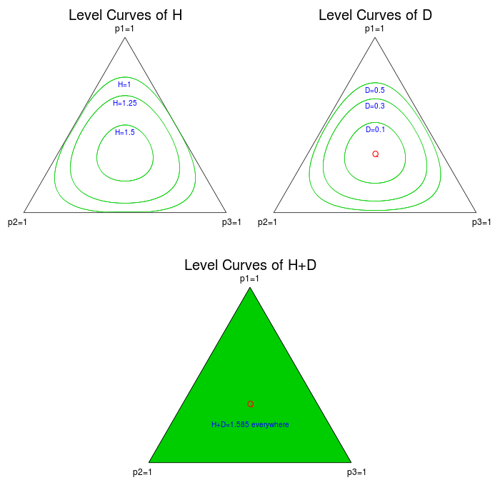
Theorem 3
The number of outcomes in the type class of $P$ is bounded by $2^{n H(P)}$.
Proof
The number of outcomes in any type class has nothing to do with the true distribution $Q$. Therefore, without loss of generality, let us assume that $P = Q$ so that $D(P \, \Vert Q)=0$. By Theorem 2, the probability of each outcome is $2^{-n H(P)}$. If the number of outcomes in the class were greater than $2^{n H(P)}$, then the total probability of that class would be greater than 1 which is a contradiction. $\square$
In fact, C&T show the stronger result that the number of outcomes in $T(P)$ is approximately $2^{n H(P)}$ for large $n$. The entropy level curves plotted above can give us an idea how many outcomes there are at various points in the simplex.
Theorem 4
The probability that $\Px$ equals $P$ is bounded by $2^{-n D(P \, \Vert Q)}$.
Proof
Each outcome in the type class is equally probable. Therefore, the probability that an outcome in the class occurs is simply the product of the probability of each outcome in $T(P)$ and the number of outcomes in $T(P)$. Theorem 2 tells us that the probability of each outcome is $2^{-n (H(P) + D(P \, \Vert Q))}$. Theorem 3 bounds the number of outcomes by $2^{n H(P)}$. Therefore, the total probability is bounded by the product of these, which simplifies to $2^{-n D(P \, \Vert Q)}$. $\square$
Again, C&T show the stronger result that the probability that $\Px$ equals $P$ is approximately $2^{-n D(P \, \Vert Q)}$ for large $n$. The level curves of relatively entropy plotted above show us about how probable different regions of the simplex are.
Typical Sets (Based on C&T Section 11.2)
For any true distribution $Q$, we can define the $\epsilon$-typical set
Lemma 1
For any $\epsilon$, the probability that $\Px$ is in $T_Q^\epsilon$ goes to 1 as $n \rightarrow \infty$.
Proof
From C&T page 356
$\square$
Theorem 5
As $n$ goes to $\infty$, $D(\Px \Vert Q) \rightarrow 0$ with probability 1.
Proof
(From C&T page 356) The probability of the compliment of the typical set is the probability that $D(\Px \Vert Q) > \epsilon$. Notice from the proof of Lemma 1 that this probability is bounded by $2^{-n \left( \epsilon - m \frac{\log(n+1)}{n} \right)}$. If we sum these probabilities over all $n$, we get a finite value. Therefore, by the Borel-Cantelli lemma, the probability that the event ${ D(\Px \Vert Q) > \epsilon }$ occurs an infinite number of times is 0. In other words, with probability 1, $D(\Px \Vert Q)$ will be greater than any given $\epsilon$ only finitely many times, meaning that $D(\Px \Vert Q) \rightarrow 0$. $\square$
Another notion of typicality is also useful. We define the strongly typical set
Theorem 6
The probability of the strongly typical set goes to 1 as $n$ goes to $\infty$.
Proof
We know from Theorem 5 that $D(\Px \Vert Q) \rightarrow 0$ on a set of probability 1; let us call this set $F$. By Pinsker’s inequality, the total variation distance from $\Px$ to $Q$ must also go to 0 on $F$. This distance can be expressed as $\sum_{a \in A} \vert \Px(a) - Q(a) \vert$. For the sum to go to zero, each component must go to zero, so for all $a \in A$, $\vert \Px(a) - Q(a) \vert \rightarrow 0$.
The other condition we need for strong typicality is that $\Px(a) = 0$ for all $a$ that have $Q(a)=0$. The probability of any sequence that contains such an $a$ is zero, so this condition is is clearly true on some set $G$ with probability 1. The intersection of $F$ and $G$ has probability 1, and all outcomes in this intersection are eventually in the strongly typical set. Therefore, the probability of the strongly typical set goes to 1. $\square$
For comparison, I have plotted the typical set and strongly typical set with $\epsilon=.15$ in the $m=3$ case.
maxDiff <- function(p1, p2, p3 = 1 - p1 - p2, q1, q2, q3 = 1 - q1 - q2) {
    # Maximum absolute difference between components
    p <- c(p1, p2, p3)
    q <- c(q1, q2, q3)
    return(max(abs(p - q)))
}

q1 <- 1/2
q2 <- 1/3
d <- 0.15
png("TypicalSets.png", height = 350, width = 700)
grid.newpage()
pushViewport(viewport(x = 0, w = 0.5, y = 0, just = c("left", "bottom")))
pushViewport(viewport(w = unit(10, "cm"), h = unit(10 * sqrt(3)/2, "cm")))
drawSimplex()
grid.text("Typical Set", 0.5, 1.13, gp = gpar(fontsize = 20))
grid.text("Q", simplexTransform(q1, q2), q1, default.units = "native",
          gp = gpar(col = 2))
l <- levelCurve(D, q1 = q1, q2 = q2, d = d)
p1 <- l[, 1]
p2 <- simplexTransform(l[, 1], l[, 2])
m <- length(p1)
grid.segments(p2, p1, p2[c(2:m, 1)], p1[c(2:m, 1)], gp = gpar(col = 3))
popViewport(1)
popViewport(1)
pushViewport(viewport(x = 0.5, y = 0, w = 0.5, just = c("left", "bottom")))
pushViewport(viewport(w = unit(10, "cm"), h = unit(10 * sqrt(3)/2, "cm")))
drawSimplex()
grid.text("Strongly Typical Set", 0.5, 1.13, gp = gpar(fontsize = 20))
e <- d/3
p1 <- c(q1+e, q1+e, q1, q1-e, q1-e, q1)
p2 <- c(q2, q2-e, q2-e, q2, q2+e, q2+e)
grid.polygon(x=simplexTransform(p1, p2), y=p1,
             gp=gpar(col=3, lty=3))
grid.text("Q", simplexTransform(q1, q2), q1, default.units = "native",
          gp = gpar(col = 2))
#l <- levelCurve(maxDiff, q1 = q1, q2 = q2, d = d/3)
#p1 <- l[, 1]
#p2 <- simplexTransform(l[, 1], l[, 2])
#m <- length(p1)
#grid.segments(p2, p1, p2[c(2:m, 1)], p1[c(2:m, 1)], gp = gpar(col = 3, lty = 3))
popViewport(1)
popViewport(1)
dev.off()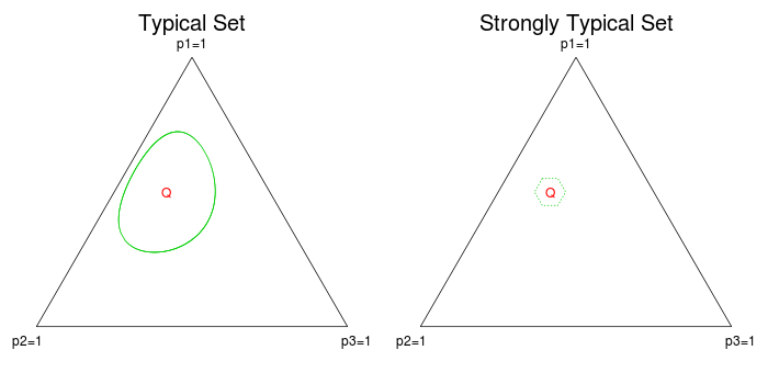
Large Deviations (Based on C&T Section 11.4)
One of the most fundamental results in large deviations theory is Sanov’s Theorem. It tells us about the probabilities of rare events as $n$ gets large.
When the support of $X_i$ is discrete or a Polish space, Sanov’s Theorem requires $E$ to be a convex and weakly-closed set in the space of possible distributions for $X_i$. However, in the finite setting that we have been dealing with, a similar theorem holds with no such requirements on $E$.
We can use the method of types tools developed above to prove a simplified version of Sanov’s result for any rare event $E$ in the probability simplex.
Finite Sanov’s Theorem (Abridged)
If $E$ is a subset of the probability simplex, then $\P E$ is bounded by $(n+1)^m 2^{-n D( E \, \Vert Q )}$, where
Proof
This proof follows almost the exact same format as that of Lemma 1 above. It is from page 363 of C&T. Let $\Pn$ be the set of possible empirical distributions when there are $n$ observations.
$\square$
Using their lower bound for the total probability of a type class, C&T show the more powerful result that if $E$ is the closure of its interior, then $\P E \approx 2^{-n D(E \, \Vert Q) + o(n)}$ for large $n$.
Also, other formulations of Sanov’s Theorem would take $D( E \, \Vert Q )$ to be the relative entropy $D( P^* \Vert Q )$, where $P^*$ is the information projection of $Q$ onto $E$. However, without assuming that $E$ is convex or weakly-closed, we are not guaranteed existence or uniqueness of an information projection.
blog comments powered by Disqus