An Unbiased Estimator for Normal Standard Deviation Math, CS, Data

When estimating the variance of a sequence $X_1, \ldots, X_n$ of i.i.d. $N(\mu, \sigma^2)$ random variables, a common procedure is to use the unbiased estimator $S^2 := \frac{V}{n-1}$, where $V := \sum(X_i - \bar{X})^2$. Note that $V/\sigma^2$ is distributed $\chi^2_{n-1}$ and that its expectation is $n-1$. Therefore, letting $k := n-1$ be the degrees of freedom,

However, what should we do if we wish to estimate $\sigma$, the standard deviation? One idea is to simply take the square root of $S^2$. Its expectation is $\frac{\sigma}{\sqrt{k}} \E \sqrt{V/\sigma^2}$. To determine this quantity, we can find the distribution of $\sqrt{V/\sigma^2}$, which is a square-root transformed chi-squared random variable. Let $f$ be the density for $\chi^2_k$. Because the transformation is monotonic, the transformed density is simply

The following plot demonstrates the two densities for the $k=9$ case. The original density is in black, while the transformed density is in red.

g <- function(y, k) {
    return(2 * y * dchisq(y^2, df = k))
}

k <- 9
grid <- seq(0, 25, 0.1)
plot(grid, dchisq(grid, df = k), type = "l", ylim = c(0, 0.55), ylab = "density", 
     xlab = "x")
lines(grid, sapply(grid, g, k = k), col = 2, lty = 2)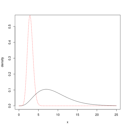

The expectation of the transformed random variable is

$\dagger$ Note that the integral was determined by inspecting the form of the original density $g$.

Therefore, the expectation of $\sqrt{S^2}$ is $\sigma \frac{\Gamma(k/2+1/2)}{\Gamma(k/2) (k/2)^{1/2}}$. We can see that this estimator is biased; it underestimates the true standard deviation. However, the estimator is consistent because the factor multiplying $\sigma$, let’s call it $b(k)$, goes to 1 as $k \rightarrow \infty$.

b <- function(k) {
    if(k > 342) return(1) # Avoid computational problems
    return(gamma(k/2+.5)/gamma(k/2)/sqrt(k/2))
}

grid <- seq(0, 25, 0.1)
plot(grid, sapply(grid, b), type = "l", ylab = "b", xlab = "k")

abline(h = 1, col = 3, lty = 2)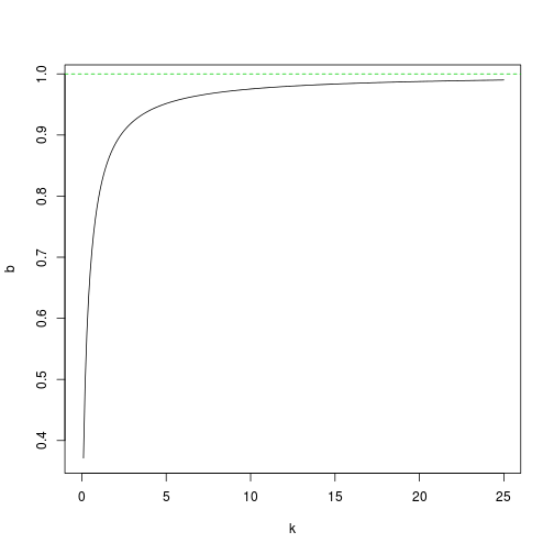

An unbiased estimator of $\sigma$ is

which simplifies to $\frac{\Gamma(k/2)}{\Gamma(k/2+1/2)} \sqrt{V/2}$.

The code below simulates normal observations (sample size $n=20$) and computes the biased and unbiased estimators, for a range of different standard deviations. It repeats the process ten thousand times and presents the average estimates.

VarEst <- function(x) {
    return(sum((x - mean(x))^2)/(length(x) - 1))
}

n <- 20
sd <- 2:10

nsim <- 10000
est <- matrix(NA, length(sd), nsim)
for (i in 1:nsim) {
    x <- matrix(rnorm(length(sd) * n, 0, sd), length(sd), n)
    est[, i] <- sqrt(apply(x, 1, VarEst))
}

sqrtssq <- apply(est, 1, mean)
results <- cbind(sd, sqrtssq, sqrtssq/b(n - 1))
colnames(results) <- c("standard deviation", "biased est", "unbiased est")

results


##       standard deviation biased est unbiased est
##  [1,]                  2      1.971        1.997
##  [2,]                  3      2.965        3.005
##  [3,]                  4      3.951        4.004
##  [4,]                  5      4.932        4.997
##  [5,]                  6      5.923        6.002
##  [6,]                  7      6.929        7.021
##  [7,]                  8      7.903        8.008
##  [8,]                  9      8.878        8.996
##  [9,]                 10      9.852        9.982

Note that this analysis was only concerned with bias and did not compare estimators based on other criteria, such as mean squared error. But it can be shown that our unbiased estimator is the MVUE. Also, note that when $n$ is large, the two estimators are practically equal.

Published

Tags

• math 9