Comparing k-Nearest Neighbors and Linear Regression Math, CS, Data
This is a simple exercise comparing linear regression and k-nearest neighbors (k-NN) as classification methods for identifying handwritten digits. It’s an exercise from Elements of Statistical Learning. The training data and test data are available on the textbook’s website.
The data come from handwritten digits of the zipcodes of pieces of mail. We would like to devise an algorithm that learns how to classify handwritten digits with high accuracy.
There are 256 features, corresponding to pixels of a sixteen-pixel by sixteen-pixel digital scan of the handwritten digit. The features range in value from -1 (white) to 1 (black), and varying shades of gray are in-between.
The training data set contains 7291 observations, while the test data contains 2007.
The first column of each file corresponds to the true digit, taking values from 0 to 9. For simplicity, we will only look at 2’s and 3’s. As a result, we can code the group by a single dummy variable taking values of 0 (for digit 2) or 1 (for digit 3).
# Read in the training data
X <- as.matrix(read.table(gzfile("zip.train.gz")))
y2or3 <- which(X[, 1] == 2 | X[, 1] == 3)
X.train <- X[y2or3, -1]
y.train <- X[y2or3, 1] == 3

# Read in the test data
X <- as.matrix(read.table(gzfile("zip.test.gz")))
y2or3 <- which(X[, 1] == 2 | X[, 1] == 3)
X.test <- X[y2or3, -1]
y.test <- X[y2or3, 1] == 3
Just for fun, let’s glance at the first twenty-five scanned digits of the training dataset. This can be done with the image command, but I used grid graphics to have a little more control.
drawDigit <- function(x) {
    for (i in 1:16) {
        for (j in 1:16) {
            color <- gray(1 - (1 + x[(i - 1) * 16 + j])/2)
            grid.rect(j, 17 - i, 1, 1, default.units = "native",
                      gp = gpar(col = color, fill = color))
        }
    }
}

library(grid)
grid.newpage()
pushViewport(viewport(xscale = c(0, 6), yscale = c(0, 6)))
for (k in 1:25) {
    pushViewport(viewport(x = (k - 1)%%5 + 1, y = 5 - floor((k - 1)/5), width = 1,
                          height = 1, xscale = c(0, 17), yscale = c(0, 17),
                          default.units = "native"))
    drawDigit(X.train[k, ])
    popViewport(1)
}
popViewport(1)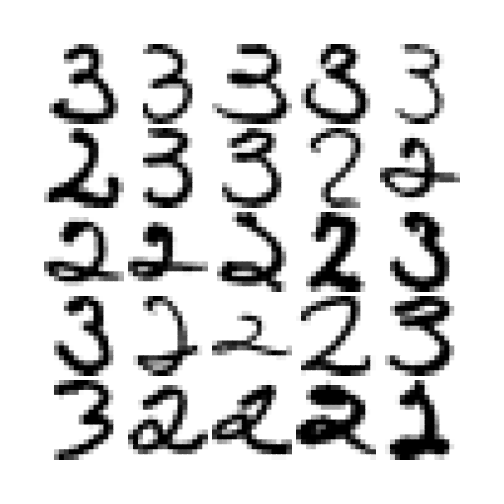
Because we only want to pursue a binary classification, we can use simple linear regression.
# Classification by linear regression
L <- lm(y.train ~ X.train)
yhat <- (cbind(1, X.test) %*% L$coef) >= 0.5
L.error <- mean(yhat != y.test)
Another method we can use is k-NN, with various $k$ values.
# Classification by k-nearest neighbors
library(class)
k <- c(1, 3, 5, 7, 15)
k.error <- rep(NA, length(k))
for (i in 1:length(k)) {
    yhat <- knn(X.train, X.test, y.train, k[i])
    k.error[i] <- mean(yhat != y.test)
}
Let’s see which method performed better.
# Compare results
error <- matrix(c(L.error, k.error), ncol = 1)
colnames(error) <- c("Error Rate")
rownames(error) <- c("Linear Regression", paste("k-NN with k =", k))
error


##                   Error Rate
## Linear Regression    0.04121
## k-NN with k = 1      0.02473
## k-NN with k = 3      0.03022
## k-NN with k = 5      0.03022
## k-NN with k = 7      0.03297
## k-NN with k = 15     0.03846


plot(c(1, 15), c(0, 1.1 * max(error)), type = "n", main = "Comparing Classifiers",
     ylab = "Error Rate", xlab = "k")
abline(h = L.error, col = 2, lty = 3)
points(k, k.error, col = 4)
lines(k, k.error, col = 4, lty = 2)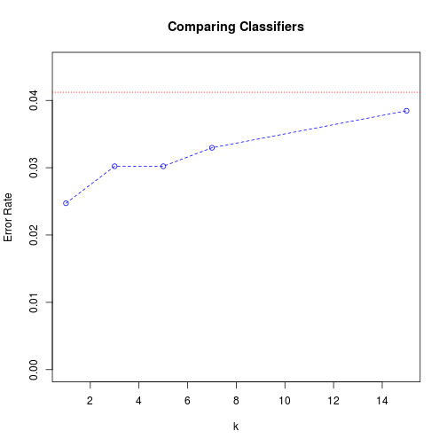
In the plot, the red dotted line shows the error rate of the linear regression classifier, while the blue dashed line gives the k-NN error rates for the different $k$ values.
For this particular data set, k-NN with small $k$ values outperforms linear regression. And among k-NN procedures, the smaller $k$ is, the better the performance is. This is because of the “curse of dimensionality” problem; with 256 features, the data points are spread out so far that often their “nearest neighbors” aren’t actually very near them.
blog comments powered by Disqus