Resolving Stein's Paradox Math, CS, Data

Assume $X$ is a vector of $n$ independent normal random variables with unknown means $\theta := (\theta_1, \ldots , \theta_n)$ and a known common variance $\sigma^2$.

The James-Stein estimator

dominates $\hat{\theta}_X := X$ as an estimator of $\theta$ with respect to norm-squared error loss. It seems strange that you would use all of the components of $X$ in your estimation of each $\theta_i$ when only one of them is related to that parameter.

This result is quite surprising to most people, and it can even mislead some of them into magical thinking.

The Magical Idea

Assume we know that $X_1 \sim N(\theta, 1)$, and we wish to estimate $\theta_1$. The common-sense approach is to estimate $\theta_1$ by $X_1$. But because we’re familiar with Stein’s phenomenon, we may decide to try a clever trick to improve the estimation:

1. Gather unrelated data.
2. Use Stein shrinkage.
3. Improve risk?

Gather Unrelated Data

The simplest way to do this would be to use a computer to generate two standard normal observations $X_1$ and $X_2$ (i.e. $\theta_2 = \theta_3 = 0$).

Use Stein Shrinkage

Our estimator is

Improve Risk?

Overall Risk

Using Stein’s Lemma, we can compute the overall risk of this estimator to be

as shown in Essentials of Statistical Inference by Young and Smith. Holding $\theta_2$ and $\theta_3$ fixed at zero, we can consider this risk to be a function of only $\theta_1$. The expectation term is equivalent to an expectation of $1/Y$ where $Y$ is noncentral chi-squared distributed with three degrees of freedom and noncentrality parameter $\theta_1^2$.

So in fact, $R(\theta)$ only depends on $\theta_1^2$. Let us define $B(\theta_1^2) := \E (1/\Vert X \Vert^2)$. For any given $\theta_1^2$, we can solve it numerically by integrating over the appropriate noncentral chi-squared density. Let us plot this risk function against $\theta_1^2$.

B <- function(t) {
    # Note: This integral can be solved analytically
    fun <- function(x) {
        dchisq(x, df = 3, ncp = t)/x
    }
    return(integrate(fun, 0, Inf)$value)
}

grid <- seq(0, 25, by = 0.25)
b <- sapply(grid, B)
R <- 3 - b
plot(c(0, 25), c(2, 3), type = "n", ylab = "Risk",
     xlab = expression(theta[1]^2))
abline(h = 3, lty = 2, col = 3)
lines(grid, R)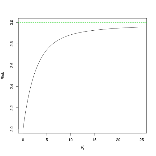

For reference, the ordinary estimator’s constant risk of 3 is plotted as well. We can see that this James-Stein estimator certainly achieves a lower overall risk. But we don’t actually care about our estimates of $\theta_2$ or $\theta_3$. Let’s look at the only risk that matters: the component risk function for $\theta_1$.

Component Risks

The overall risk function is the sum of three component risk functions

Each component risk is

defining $C_i(\theta_1^2) := \E X_i^2 / \Vert X \Vert^4$. (In our scenario, this expectation only depends on $\theta_1^2$.) One can verify that the three component risks do indeed add up to the overall risk.

To find $C_1$, consider a non-central chi-squared random variable $V$ with one degree of freedom and non-centrality parameter $\theta_1^2$. Let $W$ be an central chi-squared random variable, independent of $V$, with two degrees of freedom. Then the value of $C_1$ is equal to the expectation of $V/(V+W)^2$. This can be computed with a double integral.

A similar argument gives us $C_2$. The difference is that we want to find the expectation of $W/(V+W)^2$, where $W$ now has only one degree of freedom and $V$ now has two. By symmetry, we can see that $C_3$ must be equal to $C_2$ for all $\theta_1^2$.

Let’s look at a plot of the first component risk.

C1 <- function(t) {
    # Note: Order of integration is important here
    # to avoid computational problems
    inner <- function(v, w)
      dchisq(v, df = 1, ncp = t) * dchisq(w, df = 2) * v/(v + w)^2
    outer <- function(w) sapply(w, function(w) integrate(inner, w = w, 0, Inf)$value)
    return(integrate(outer, 0, Inf)$value)
}

R1 <- 1 - 2 * b + 5 * sapply(grid, C1)
plot(c(0, 25), c(0.6, 1.3), type = "n", ylab = "Risk 1",
     xlab = expression(theta[1]^2))
abline(h = 1, lty = 2, col = 2)
lines(grid, R1)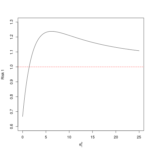

If $\theta_1$ is close enough to zero, then your risk decreases. Otherwise, you are actually increasing your risk by engaging in this scheme.

The only reason the overall risk is less than 3 everywhere is that the other two components’ risks are far enough below 1 to make up for the additional risk in the first component.

C2 <- function(t) {
    inner <- function(w, v)
      dchisq(v, df = 2, ncp = t) * dchisq(w, df = 1) * w/(v + w)^2
    outer <- function(v) sapply(v, function(v) integrate(inner, v = v, 0, Inf)$value)
    return(integrate(outer, 0, Inf)$value)
}

R2 <- 1 - 2 * b + 5 * sapply(grid, C2)
plot(c(0, 25), c(0.6, 1), type = "n", ylab = "Risk 2",
     xlab = expression(theta[1]^2))
abline(h = 1, lty = 2, col = 2)
lines(grid, R2)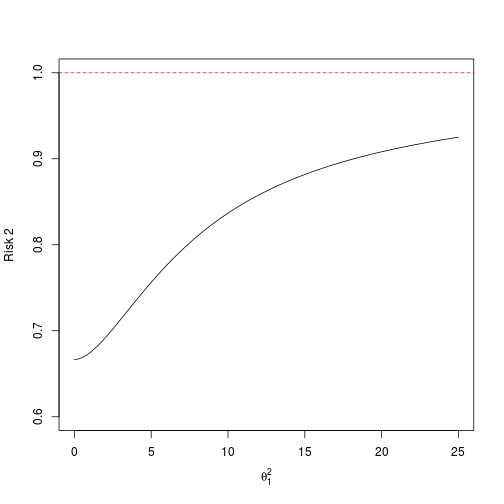

The reason this estimator seems to work so well for $\theta_2$ and $\theta_3$ is because it is shrinking toward zero, which is their actual mean. If we allowed their means to vary, we would not necessarily see this uniform improvement.

Generalization

Let’s think more generally about the $n=3$ case described above, allowing $\theta \in \R^3$. For simplicity, we can actually just consider $(\theta_1^2, \theta_2^2, \theta_3^2) \in [0,\infty)^3$, because the squared means are sufficient in determining the risks.

Earlier, we held $\theta_2^2 = \theta_3^2 = 0$ and varied $\theta_1^2$. This showed us the risk functions as we travelled along the $\theta_1^2$. By symmetry, we can get similar pictures when we travel along either of the other axes.

As a final exercise, I want to consider the behavior of the risk functions along the $(1, 1, 1)$ direction (i.e. $\theta_1^2 = \theta_2^2 = \theta_3^2$).

To compute the risk of the first component, we revisit the original formulation of $V$ and $W$, with the exception that $W$ now has noncentrality parameter $2 \theta_1^2$.

C <- function(t) {
    inner <- function(w, v)
      dchisq(v, df = 2, ncp = 2 * t) * dchisq(w, df = 1, ncp = t) * w/(v + w)^2
    outer <- function(v) sapply(v, function(v) integrate(inner, v = v, 0, Inf)$value)
    return(integrate(outer, 0, Inf)$value)
}

b3 <- sapply(3 * grid, B)
R1 <- 1 - 2 * b3 + 5 * sapply(grid, C)
plot(c(0, 25), c(0.6, 1), type = "n", ylab = "Risk 1",
     xlab = expression(theta[1]^2))
abline(h = 1, lty = 2, col = 2)
lines(grid, R1)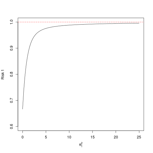

In the subspace we are limiting ourselves to, the first component risk looks the same when plotted against any axis. Furthermore, by symmetry, the two other component risk functions are identical to the first.

Looking at the plot, it seems that maybe we have found a magic trick after all. It appears that we have an estimator of $\theta_1$ that dominates $X$. (This can’t be true, of course, because it is well-known that $X$ is admissible.) In fact, this “estimator” is only an illusion. The decision procedure requires generating $X_2$ and $X_3$ from $N(\theta_1, 1)$. This is a different procedure for each value of $\theta_1^2$, so we can’t consider it a well-defined estimator.

Published

Tags

• math 9