Rejection Sampling Math, CS, Data
An earlier post discussed inverse transform sampling. Another way to sample from a known pdf is to use rejection sampling. First, find a density $f$ that you can sample from and that dominates the density of interest $h$. Next, find a value $M$ such that $Mf \geq h$ (i.e. $M f(x) \geq h(x) \; \forall x \in \R$). Preferably, you should find the smallest such $M$ value, to make the algorithm as fast as possible. Finally, sample from $f$, and keep each sample value $x_i$ with probability $h(x_i)/(Mf(x_i))$.
Example Using Exponential Distribution
Suppose, as in the previous post, we wish to sample from the pdf
For this analysis, let’s assume the parameter $m$ is $.3$. To perform our rejection sampling, let’s use a shifted exponential distribution as our source of random values (credit: Jay Emerson).
h <- function(x, m = 0.3) {
    if (x >= m & x <= 1)
        return(2 * m^2/(1 - m^2)/x^3)
    return(0)
}

m <- 0.3
grid <- seq(m, 1.5, length.out = 1000)
plot(grid, sapply(grid, h), type = "l", xlim = c(m, 1.5), xlab = "x", ylab = "density",
    main = paste("h and", m, "+ Exp(1)"))
lines(grid, dexp(grid - m), col = 2)
legend(1, 5.5, c("h", paste(m, "+ Exp(1)")), col = 1:2, lty = 1)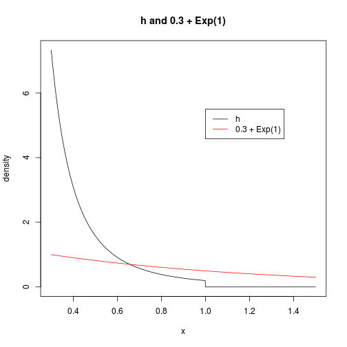
Now, we want to find the smallest $M$ such that $M$ times our exponential density is greater than $h$ for all $x$. We also have the freedom to adjust the exponential rate parameter, if we want. A fundamental result in rejection sampling is that the overall acceptance rate of a procedure is exactly equal to $1/M$. Therefore, let’s try to find the rate parameter $\lambda>0$ for which the smallest $M$ will suffice. This will give us the procedure that has the highest acceptance rate (fewest “wasted” trials) of any procedure in this shited exponential class.
Our shifted exponential density will be of the form $f(x; \lambda) = \lambda e^{-\lambda (x-m)} \I{x \geq m}$. Assuming $x \in [m, 1]$, we need $M$ to satisfy
For a given $\lambda$, we want $M$ to be the smallest value satisfying the above condition, so we will let $M$ be the supremum over $x$ of the expression on the right-hand side, which I will call $g(x, \lambda)$. By differentiating $g$ with respect to $x$, we can see that it is convex on the interval we’re considering; therefore, its maximum must occur at an endpoint. Now, let’s define
Because the supremum occurs at an endpoint, the only two possibilities for $S(\lambda)$ are $g(m; \lambda)$ and $g(1; \lambda)$. By substituting these two $x$ values and comparing, it can be shown that
By differentiating with respect to $\lambda$, we find that $S$ is minimized at $\lambda = -\tfrac{3}{1-m} \log m$ which is approximately $5.16$ when $m=.3$. This corresponds to an $M$ value of about 1.42 and an acceptance rate of about 70 percent. The acceptance rate as a function of $\lambda$ is plotted below, along with a dotted line showing simulated results.
S <- function(lambda, m = 0.5) {
    if (lambda < -3/(1 - m) * log(m))
        return((2 * m^2/(1 - m^2))/(lambda * m^3))
    return((2 * m^2/(1 - m^2)) * exp(lambda * (1 - m))/lambda)
}

grid <- seq(0.1, 10, length.out = 100)
M <- sapply(grid, S)
plot(grid, 1/M, type = "l", col = 2, xlab = "lambda", ylab = "probability",
    main = "Acceptance Rate")

N <- 1000
results <- rep(NA, length(grid))
for (i in 1:length(grid)) {
    raw <- m + rexp(N, grid[i])
    u <- runif(N, max = M[i] * dexp(raw - m, grid[i]))
    results[i] <- sum(u <= sapply(raw, h))/N
}
lines(grid, results, col = 3, lty = 3)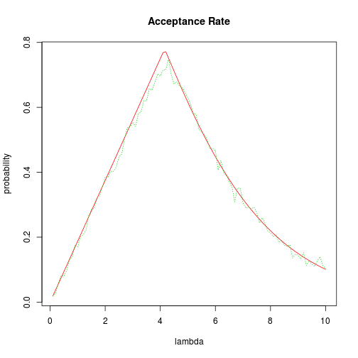
It is possible that different rate parameters cause the random number generator to take different amounts of time. However, after a quick check, this question seems unlikely to be worth pursuing. The simulation below shows that Exp(1) is generated at basically the same rate as Exp(5.16).
nsim <- 1e+05
rates <- c(1, 5.16)
repetitions <- 5
results <- matrix(NA, nrow = repetitions, ncol = length(rates))
colnames(results) <- paste("rate:", rates)
for (i in 1:repetitions) {
    for (j in 1:length(rates)) {
        results[i, j] <- system.time(rexp(nsim, rates[j]))[3]
    }
}
results


##      rate: 1 rate: 5.16
## [1,]   0.027      0.027
## [2,]   0.027      0.028
## [3,]   0.026      0.027
## [4,]   0.027      0.027
## [5,]   0.027      0.026
Therefore, we can be satisfied that using $\lambda=5.16$ is about as well as we can do in drawing from $h$ via an exponential rejection sampling.
Repeat Using Histograms
Another way to use rejection sampling for a density with bounded support is by drawing from a histogram. First, you construct a histogram shape that covers the density of interest, then divide each rectangle’s area by the total area to normalize to a probability mass function (pmf) for the bins. Next, draw a bin according to that pmf. Uniformly sample a horizontal and vertical position with that bin’s rectangle. If this point is below the density of interest, then keep the $x$ value.
We will apply this method to draw from $h$. First, here is a picture of the true density and the histogram-like density if we use ten bins, for example.
grid <- seq(m, 1, length.out = 100)
plot(grid, sapply(grid, h), type = "l", ylim = c(0, 7.4), xlab = "x",
     ylab = "density", main = "Density of h and Scaled Histogram")

r <- 10  # number of bins
binpoints <- seq(m, 1, length.out = r + 1)
binheights <- sapply(binpoints[1:r], h)

# visualizing the process
picx <- sort(c(binpoints[1:r], binpoints[2:length(binpoints)]))
picy <- rep(binheights, each = 2)
lines(picx, picy, col = 2)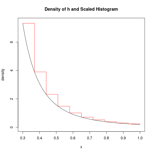
We will call the number of bins $r$ (for refinement). It is clear that we can drive the acceptance probability arbitrarily close to 1 by increasing $r$. However, there is a trade-off because the larger $r$ is, the longer it takes to generate each point. We will look for the $r$ that optimizes overall speed. The rsample.h function below samples from $h$ using this histogram method with a given $r$ value.
rsample.h <- function(r, N = 1000) {
    binwidth <- (1 - m)/r
    grid <- seq(m, 1, length.out = r + 1)
    binheights <- sapply(grid[1:r], h)
    binprobs <- binheights/sum(binheights)

    s <- sample.int(r, N, replace = T, prob = binprobs)
    x <- m + (s - 1) * binwidth + runif(N, 0, binwidth)
    return(x[which(runif(N, 0, binheights[s]) - sapply(x, h) <= 0)])
}
Now, we try out a series of $r$ values to determine the time required as a function of $r$.
r <- 1:10 * 200
ntime <- function(n, f, ...) {
    return(system.time(f(n, ...))[3])
}

times <- sapply(r, ntime, f = rsample.h)

plot(r, times)
fit <- lm(times ~ r)$coeff
fit <- signif(fit, 3)
print(paste("The time (in seconds) required to generate 1000 points is about",
    fit[1], "+", fit[2], "* r."))


## [1] "The time (in seconds) required to generate 1000 points is about 0.0435 + 4.31e-05 * r."


abline(fit, col = 2)
The algorithm is linear in $r$. The expected time required to reach 1000 \textcal{accepted} draws is approximately the time required to generate 1000 points divided by the acceptance rate. We could find the acceptance rate by conditioning on the bin selected and finding the conditional acceptance rate for each bin. But it is simpler to just use the result invoked earlier: the acceptance rate is $1/M$, where $M$ is the sum of the rectangle areas. In fact, I wrote code for both; the rejectionprob function does it “the hard way,” while acceptanceprob uses the easy method. As a sanity check, you can confirm that the sum of these two functions is 1 for any $r$.
rejectionprob <- function(r) {
    binwidth <- (1 - m)/r
    grid <- seq(m, 1, length.out = r + 1)
    binheights <- sapply(grid[1:r], h)
    binprobs <- binheights/sum(binheights)
    binareas <- binheights * binwidth
    rejection <- function(x, i) {
        return(binheights[i] - sapply(x, h))
    }
    p <- 0
    for (i in 1:r) {
        rejectarea <- integrate(rejection, m + (i - 1) * binwidth, m + i * binwidth,
            i = i)$value
        p <- p + binprobs[i] * rejectarea/binareas[i]
    }
    return(p)
}

acceptanceprob <- function(r) {
    binwidth <- (1 - m)/r
    grid <- seq(m, 1, length.out = r + 1)
    binheights <- sapply(grid[1:r], h)
    binareas <- binheights * binwidth
    return(1/sum(binareas))
}
We want to find the $r$ value that minimizes number-generating time divided by acceptance rate. Because it is a discrete problem, all we need to do is evaluate the possible $r$ values.
expectedtime <- function(r) {
    time <- fit %*% c(1, r)
    return(time/acceptanceprob(r))
}

r <- 1:200
exptimes <- sapply(r, expectedtime)
plot(r, exptimes, type = "l", col = 2, xlab = "r (number of bins)", ylab = "seconds",
    main = "Expected Time to Draw 1000 from h")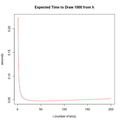
which.min(exptimes)


## [1] 51
Comparing Speeds of the Exponential and Histogram Algorithms
Lastly, let’s compare the two rejection sampling methods described above. Using the histogram method we can make the acceptance probability arbirarily close to 1 simply by increasing the number of bins. That may make it seem like this method is superior to the exponential one. However, the histogram method requires one extra randomization step, so it could still be worse overall. Let’s see how the best exponential method and the best histogram method match up head-to-head in sampling from $h$.
rsample.h.optimal <- function(N = 1e+05) {
    # returns amount of time required per N accepted points using optimal
    # parameter values
    r <- 51
    time <- system.time({
        binwidth <- (1 - m)/r
        grid <- seq(m, 1, length.out = r + 1)
        binheights <- sapply(grid[1:r], h)
        binprobs <- binheights/sum(binheights)

        s <- sample.int(r, N, replace = T, prob = binprobs)
        x <- m + (s - 1) * binwidth + runif(N, 0, binwidth)
        numaccepted <- sum(runif(N, 0, binheights[s]) - sapply(x, h) <= 0)
    })[3]
    return(1e+05 * time/numaccepted)
}

esample.h.optimal <- function(N = 1e+05) {
    # returns amount of time required per N accepted points using optimal
    # parameter values
    lambda <- 5.16
    M <- S(lambda)
    time <- system.time({
        raw <- m + rexp(N, lambda)
        u <- runif(N, max = M * dexp(raw - m, lambda))
        numaccepted <- sum(u <= sapply(raw, h))
    })[3]
    return(1e+05 * time/numaccepted)
}

methods <- c("esample.h.optimal", "rsample.h.optimal")
repetitions <- 5
results <- matrix(NA, repetitions, length(methods))
colnames(results) <- c("exponential", "histogram")
for (i in 1:repetitions) {
    order <- sample.int(length(methods), length(methods))
    for (j in order) {
        results[i, j] <- get(methods[j])()
    }
}
print("Amount of time needed to reach 100,000 accepted values:")


## [1] "Amount of time needed to reach 100,000 accepted values:"


results


##      exponential histogram
## [1,]       7.196     5.133
## [2,]       6.331     3.943
## [3,]       7.247     3.925
## [4,]       6.405     3.883
## [5,]       6.304     3.883
The histogram method consistently outperforms the exponential method, at least with the implementation I coded up. And as an added bonus, the histogram method can be packaged as a general-purpose function that doesn’t require any thought to use, especially when the density is monotonic or monomodal. It would take some extra code and extra computation to make the function choose a near-optimal $r$ value, but that could be accomplished as well.
Unfortunately, the histogram method requires the density of interest to have bounded support. Although, in practice, if you had a density with unbounded support, you could cut it off way out on the tails without changing your results.
blog comments powered by Disqus