Volatility Profiles Math, CS, Data

Constant Volatility over Small Intervals

Stock prices are often modeled by Geometric Brownian Motion. Each stock is assumed to have a volatility parameter that is roughly stable over time frames on the order of, say, a year. In practice, stock prices tend to change much more rapidly at the beginning and end of each trading day than they do in the middle. To analyze intra-day volatilities, we need to use a more general diffusion model that allows the volatility to depend on $t$. I will refer to a stock’s daily volatility pattern as its “volatility profile.”

In theory, one could compute volatility estimates over arbitrarily small time intervals. However, the more you zoom in, the less “GBM-like” stock prices are. For our analysis, we broke each trading day ($T=6.5$ hours) into seventy-eight five-minute ($l=5$ minutes) intervals. On day $i$, represent a stock price in terms of a standard Brownian Motion $W_i$ by

We define $n=T/l=78$ random variables, one for each interval:

As a first attempt, we are assuming $\sigma(j l) \approx \sigma((j-1)l) \approx \sigma(j l - l/2)$, that is, volatility is nearly constant over small intervals. For a given stock, each $X_{i,j}$ is normal with mean $l \mu$ and variance approximately $l$ times $\sigma^2(j l - l/2)$ (henceforth abbreviated to $\sigma^2$), and they are independent of each other.

Assume we have data for $m$ trading days. The random variable

has an approximately $\chi^2_{m-1}$ distribution, so the standard unbiased estimator of $\sigma^2$ is $S^2/l$, where $S^2 := \sum(X_{i,j} - \bar{X}_j)^2/(m-1)$. The mean-squared error of this estimator is equal to its variance

Refer to earlier posts for an analysis of this estimator, along with a comparison to other estimators. Yet another post describes how to estimate volatility rather than squared volatility.

Unfortunately, after glancing at some plots, the assumption of nearly constant volatility over five-minute intervals seems entirely untenable. Often, a volatility seems to change by a large proportion over the course of five minutes. Typical plots showing this can be found in the another article.

Linearly Changing Volatility over Small Intervals

After realizing this problem, I devised a more plausible assumption: the change in volatility over any five-minute interval is approximately linear. Let $V(t)$ be a process whose natural logarithm is a diffusion with linearly changing $\sigma(t)$. That is,

Let us zero in on the complicated part of this expression by defining $R(t) := \int_0^t (\sigma_0 + m\tau) d W(\tau)$. At any given time $t$, the diffusion $R(t)$ is locally approximated by a Brownian Motion with volatility $\sigma_0 + mt$. In other words, $R(t+\delta) - R(t)$ should approach a $N(0, (\sigma_0 + mt)^2 \delta)$ distribution as $\delta \rightarrow 0$.

By transforming the time axis of a standard Brownian Motion in just the right way, we can produce a much more familiar-looking process with this same behavior. We need to find a transformation $D$ such that $W(D(t))$ has a “volatility” of $\sigma_0 + mt$ at any time $t$. A change in time of $\delta$ from time $t$ must produce a change in $D$ by $(\sigma_0 + mt)^2 \delta$. That is, $D$ satisfies $D(t+\delta) = D(t) + (\sigma_0 + mt)^2 \delta$ in the limit. Rearranging, and taking an anti-derivative, we find that a solution is $D(t) = \sigma_0^2 t + \sigma_0 m t^2 + m^2 t^3/3$. So our final result is

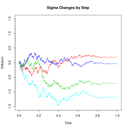
This diffusion has the same infinitesimal behavior as $R(t)$ at all times, so they are identical processes. The following simulations support this result. We will plot a diffusion on (0,1) with $\sigma(t) = 1-t$ (i.e. linear with $\sigma_0=1$ and $m=-1$). First, we generate the desired diffusion sequentially.

LinearVolDiffusion <- function(end = 1, initial = 0, mu = 0, sigma0 = 1, m = 0, 
n = 1000) {
delta <- 1/n
x <- delta * (0:n)
y <- c(initial, rep(NA, n))
for (i in 1:n) {
    t <- x[i] + delta/2
    y[i + 1] <- y[i] + mu * delta + rnorm(1, sd = (sigma0 + m * t) * sqrt(delta))
}
return(cbind(x, y))
}

plot(c(0, 1), c(-1.5, 1.5), type = "n", main = "Sigma Changes by Step", xlab = "Time", 
 ylab = "Diffusion")
for (i in 1:4) {
lines(LinearVolDiffusion(m = -1), col = i + 1)
}

Next, we generate the same diffusion using standard Brownian Motion and the $D$ transformation discovered earlier. Note that the GenerateBM function invoked below can be found in an earlier post.

right <- function(f, b = 10) {
while (f(b) < 0) b <- 10 * b
    return(b)
}

D <- function(t, sigma0 = 1, m = -1) {
    return(sigma0^2 * t + sigma0 * m * t^2 + m^2 * t^3/3)
}

Dinv <- function(x, ...) {
    sub <- function(t) D(t, ...) - x
    return(uniroot(sub, lower = 0, upper = right(sub))$root)
}

plot(c(0, 1), c(-1.5, 1.5), type = "n", main = "SBM with Transformed Time Axis", 
    xlab = "Time", ylab = "Diffusion")
for (i in 1:4) {
    b <- GenerateBM(end = D(1))
    lines(sapply(b[, 1], Dinv), b[, 2], col = i + 1)
}

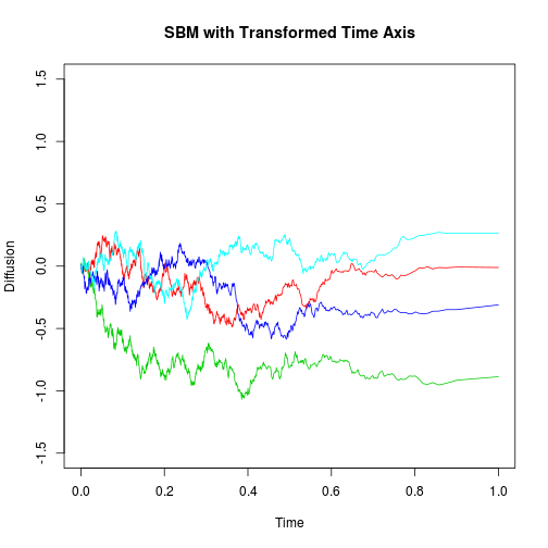
The resemblance between the two plots gives us some reassurance that our results are correct.

Now consider the distribution of $\log V(l)/V(0)$.

It is normally distributed with variance approximately $l (\sigma_0 + ml/2)^2$, assuming the product of $m$ and $l$, which is the change in $\sigma$ over the interval, is much smaller than one. Plots indicate that this assumption holds up quite well overall, though not perfectly; we could always use a smaller interval if necessary to make the assumption more plausible. Therefore, it is easy to see that estimating the variance from a sample of random variables with this distribution allows us to estimate $(\sigma_0 + ml/2)^2$, the squared volatility at the midpoint of the interval $(0,l)$. Likewise, it can be shown that the same process provides an estimate for the squared volatilities at the midpoints of the $n$ consecutive intervals of length $l$ from $(0,T)$.

The upshot is, we can still use the same estimator derived earlier to estimate the same quantities (midpoint $\sigma^2$ values), but now we have justified ourselves with a more believable model.

Published

Tags

• finance 6