Sampling from an Arbitrary Density Math, CS, Data
One way to sample from a known probability density function (pdf) is to use inverse transform sampling. First, you integrate the pdf to get the cumulative distribution function (cdf). Next, you find the inverse of the cdf. Finally, apply this inverse cdf to each number in a sample of Uniform(0,1) observations.
Example
Suppose we wish to sample from the pdf
The cdf is
For $u \in [0,1]$, its inverse is
Finally, we can apply the technique. Below, I generate 100 standard uniform observations and transform each using the inverse cdf.
invcdf <- function(u, m) {
    return(sqrt(m^2/(1 - (1 - m^2) * u)))
}

sample1 <- sapply(runif(100), invcdf, m = .5)
plot(density(sample1), main = "Sample Density using invcdf Function")
R Function for an Arbitrary pdf of One Variable
The R code below uses some of R’s built-in numerical methods to accomplish the inverse transform sampling technique for any arbitrary pdf that it is given. I’m sure there are some ugly pdfs for which this function wouldn’t work, but it works fine for typical densities.
endsign <- function(f, sign = 1) {
    b <- sign
    while (sign * f(b) < 0) b <- 10 * b
    return(b)
}

samplepdf <- function(n, pdf, ..., spdf.lower = -Inf, spdf.upper = Inf) {
    vpdf <- function(v) sapply(v, pdf, ...)  # vectorize
    cdf <- function(x) integrate(vpdf, spdf.lower, x)$value
    invcdf <- function(u) {
        subcdf <- function(t) cdf(t) - u
        if (spdf.lower == -Inf)
            spdf.lower <- endsign(subcdf, -1)
        if (spdf.upper == Inf)
            spdf.upper <- endsign(subcdf)
        return(uniroot(subcdf, c(spdf.lower, spdf.upper))$root)
    }
    sapply(runif(n), invcdf)
}
We can use samplepdf to sample from $h$, which we defined earlier.
h <- function(t, m) {
    if (t >= m & t <= 1)
        return(2 * m^2/(1 - m^2)/t^3)
    return(0)
}

sample2 <- samplepdf(100, h, m = .5)
plot(density(sample2), main = "Sample Density using samplepdf Function")
Computational Speed of the Algorithm
While samplepdf is convenient, it is also computationally slow. The algorithm is $O(n)$, so it is easy to estimate the time required for a large sample size. Simply fit a linear model to the times required for a set of small sample sizes, as shown below.
ntime <- function(n, f, ...) {
    return(system.time(f(n, ...))[3])
}

n <- 100 * 1:10
times <- sapply(n, ntime, f = samplepdf, pdf = h)
fit <- lm(times ~ n)$coeff
fit <- signif(fit, 2)
print(paste("The time needed (seconds) to sample from this density is about ",
    fit[1], " + ", fit[2], "*n.", sep=""))


## [1] "The time needed (seconds) to sample from this density is about 3.2 + 0.14*n."


plot(n, times, ylab = "seconds", xlab = "n", main = "Time Required", col = 3)
abline(fit, col = 2)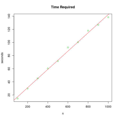
At the beginning of this document, we found the inverse cdf analytically. The R function that used this analytical result can generate a sample of size 1000 in the blink of an eye, while the samplepdf function took about two and a half minutes on my slow netbook. However, if you give the lower and upper endpoints as in samplepdf(1000, h, m = .5, spdf.lower = .5, spdf.upper = 1), the function only takes about ten seconds to run.
Another option for sampling that doesn’t require finding the inverse cdf is rejection sampling.
blog comments powered by Disqus